Automatic Control Knowledge Repository

#!/usr/bin/env python3
# -*- coding: utf-8 -*-
"""
problem solution for control problem: design a tracking controller by using nonlinear trajectory planning
to stabilize a unstable system with initial error
"""

import sympy as sp
import symbtools as st
import matplotlib.pyplot as plt
import method_trajectory_planning as tp  # noqa
from scipy.integrate import odeint
import ipydex  # noqa
import os
from ackrep_core.system_model_management import save_plot_in_dir


class SolutionData:
    pass


def rhs_for_simulation(f, g, xx, controller_func):
    """
    # calculate right hand side equation for simulation of the nonlinear system
    :param f: vector field
    :param g: input matrix
    :param xx: states of the system
    :param controller_func: input equation (trajectory)
    :return: rhs: equation that is solved
    """

    # call the class 'SimulationModel' to build the
    # 'right hand side' equation for ode
    sim_mod = st.SimulationModel(f, g, xx)
    rhs_eq = sim_mod.create_simfunction(controller_function=controller_func)

    return rhs_eq


def solve(problem_spec):
    t = sp.Symbol("t")
    planer_p2 = tp.Trajectory_Planning(
        problem_spec.YA_p2, problem_spec.YB_p2, problem_spec.t0, problem_spec.tf, problem_spec.tt
    )
    mod = problem_spec.rhs(problem_spec.ttheta, problem_spec.tthetad, problem_spec.u_F)
    planer_p2.mod = mod
    planer_p2.yy = problem_spec.output_func(problem_spec.ttheta, problem_spec.u_F)
    planer_p2.ff = mod.f  # xd = f(x) + g(x)*u
    planer_p2.gg = mod.g
    yy = planer_p2.cal_li_derivative()  # lie derivatives of the flat output
    ploy_p2 = planer_p2.calc_trajectory()  # planned trajectory of CuZn-ball
    p2_func = st.expr_to_func(t, ploy_p2[0])  # trajectory to function

    # find trajectory of Fe-ball
    p1_p2 = planer_p2.ff[3].subs(problem_spec.ttheta[1], ploy_p2[0])
    func_p1 = p1_p2 - ploy_p2[2]
    ploy_p1 = sp.solve(func_p1, problem_spec.ttheta[0])
    p1_func = st.expr_to_func(t, ploy_p1[0])

    yy_4 = yy[4].subs([(problem_spec.ttheta[0], ploy_p1[0]), (problem_spec.ttheta[1], ploy_p2[0])])
    in_output_func = yy_4 - ploy_p2[4]

    # input force trajectory
    input_f_tra = sp.solve(in_output_func, problem_spec.u_F)
    f_func = st.expr_to_func(t, input_f_tra)

    # input current trajectory
    f_c_func = problem_spec.force_current_function(problem_spec.ttheta, problem_spec.u_i)
    c_tra_func = (input_f_tra[0] - f_c_func).subs([(problem_spec.ttheta[0], ploy_p1[0])])
    input_c_tra = sp.solve(c_tra_func, problem_spec.u_i)
    current_func = st.expr_to_func(t, input_c_tra[1])

    # tracking controller
    tracking_controller = tp.Tracking_controller(yy, mod.xx, problem_spec.u_F, problem_spec.pol, ploy_p2)
    control_law = tracking_controller.error_dynamics()[0]  # control law

    # simulate the system with control law
    rhs = rhs_for_simulation(planer_p2.ff, planer_p2.gg, mod.xx, control_law)

    # original initial values : [0.0008, 0.004, 0, 0]
    res = odeint(rhs, problem_spec.xx0, problem_spec.tt2)

    solution_data = SolutionData()
    solution_data.res = res  # output values of the system
    solution_data.ploy_p1 = p1_func  # desired full transition of p1
    solution_data.ploy_p2 = p2_func  # desired full transition of p2
    solution_data.f_func = f_func  # required magnet force input
    solution_data.current_func = current_func  # required current input
    solution_data.coefficients = tracking_controller.coefficient  # coefficients of error dynamics
    solution_data.control_law = control_law  # control law function

    save_plot(problem_spec, solution_data)

    return solution_data


def save_plot(problem_spec, solution_data):
    # plotting
    plt.figure(1)  # Fe-ball p1

    plt.plot(problem_spec.tt1, solution_data.ploy_p1(problem_spec.tt1), ":", zorder=-1, label="desired full transition")
    plt.plot(
        problem_spec.tt, solution_data.ploy_p1(problem_spec.tt), "r-", linewidth=2, label="desired state transition"
    )
    plt.plot(problem_spec.tt2, solution_data.res[:, 0], "k", label="actual trajectory")
    plt.plot(0, 0.005, "rx", label="controller switch in")
    plt.title("trajectory of Fe-Ball")
    plt.xlabel("time [s]")
    plt.ylabel("position [m]")
    plt.legend(loc=4)

    plt.figure(2)  # CuZn-ball p2
    plt.plot(problem_spec.tt1, solution_data.ploy_p2(problem_spec.tt1), ":", zorder=-1, label="full transition")
    plt.plot(problem_spec.tt, solution_data.ploy_p2(problem_spec.tt), "r-", linewidth=2, label="state transition")
    plt.plot(problem_spec.tt2, solution_data.res[:, 1], "k", label="reale Trajektorie")
    plt.plot(0, 0.045, "rx", label="controller switch in")
    plt.title("trajectory of CuZn-Ball")
    plt.xlabel("time [s]")
    plt.ylabel("position [m]")
    plt.legend(loc=4)

    plt.figure(3)
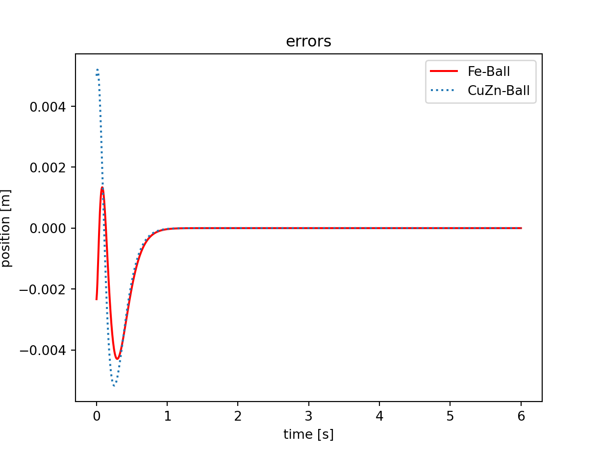
    plt.plot(problem_spec.tt2, solution_data.res[:, 0] - solution_data.ploy_p1(problem_spec.tt2), "r", label="Fe-Ball")
    plt.plot(
        problem_spec.tt2, solution_data.res[:, 1] - solution_data.ploy_p2(problem_spec.tt2), ":", label="CuZn-Ball"
    )
    plt.title("errors")
    plt.xlabel("time [s]")
    plt.ylabel("position [m]")
    plt.legend(loc=1)

    # save image
    save_plot_in_dir()