Automatic Control Knowledge Repository
You currently have javascript disabled. Some features will be unavailable. Please consider enabling javascript.Details for: "PVTOL model"
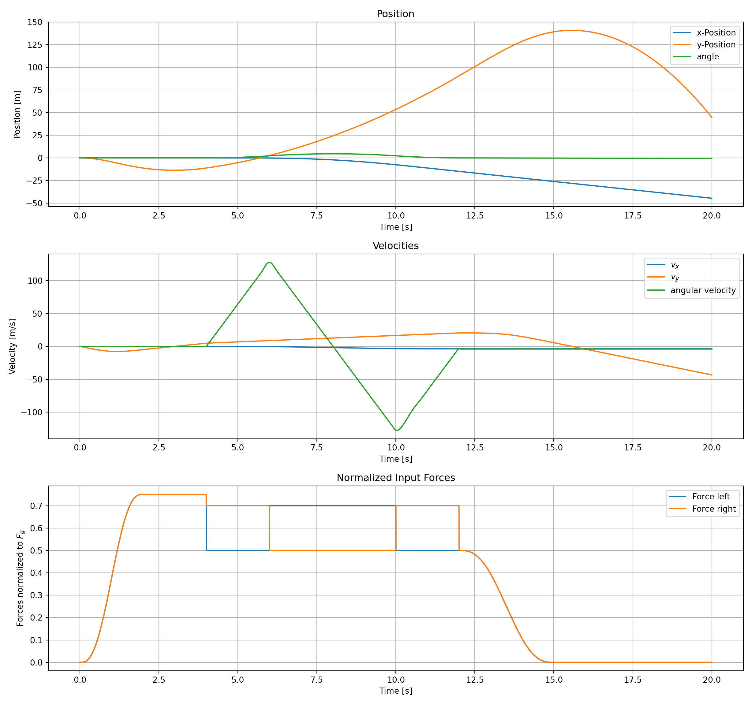
Name: PVTOL model
(Key: 8RWMB)
Path: ackrep_data/problem_solutions/PVTOL_2_Forces View on GitHub
Type: problem_solution
Short Description: creates model for PVTOL
Created: 2022-04-06
Compatible Environment: default_conda_environment (Key: CDAMA)
Source Code [ / ] solution.py
Solved Problems: PVTOL problem |
Used Methods:
Result: Success.
Last Build: Checkout CI Build
Runtime: 6.0 (estimated: 30s)
Plot:
The image of the latest CI job is not available. This is a fallback image.
Path: ackrep_data/problem_solutions/PVTOL_2_Forces View on GitHub
Type: problem_solution
Short Description: creates model for PVTOL
Created: 2022-04-06
Compatible Environment: default_conda_environment (Key: CDAMA)
Source Code [ / ] solution.py
#!/usr/bin/env python3
# -*- coding: utf-8 -*-

import matplotlib.pyplot as plt
import symbtools as st
from scipy.integrate import solve_ivp
import sympy as sp
import os
import numpy as np
from ackrep_core.system_model_management import save_plot_in_dir


class SolutionData:
    pass


def solve(problem_spec):

    rhs = problem_spec.model.get_rhs_func()

    xx_res = solve_ivp(
        rhs, [problem_spec.tt[0], problem_spec.tt[-1]], problem_spec.xx0, method="RK45", t_eval=problem_spec.tt
    )

    solution_data = SolutionData()
    solution_data.res = xx_res  # states of system

    save_plot(problem_spec, solution_data)
    return solution_data


def save_plot(problem_spec, solution_data):
    fig1, axs = plt.subplots(nrows=3, ncols=1, figsize=(12.8, 12))

    # print in axes top left
    axs[0].plot(solution_data.res.t, np.real(solution_data.res.y[0]), label="x-Position")
    axs[0].plot(solution_data.res.t, np.real(solution_data.res.y[2]), label="y-Position")
    axs[0].plot(solution_data.res.t, np.real(solution_data.res.y[4] * 180 / np.pi), label="angle")
    axs[0].set_title("Position")
    axs[0].set_ylabel("Position [m]")  # y-label Nr 1
    axs[0].set_xlabel("Time [s]")  # x-Label für Figure linke Seite
    axs[0].grid()
    axs[0].legend()

    axs[1].plot(solution_data.res.t, solution_data.res.y[1], label=r"$v_x$")
    axs[1].plot(solution_data.res.t, solution_data.res.y[3], label=r"$v_y$")
    axs[1].plot(solution_data.res.t, solution_data.res.y[5] * 180 / np.pi, label="angular velocity")
    axs[1].set_title("Velocities")
    axs[1].set_ylabel("Velocity [m/s]")
    axs[1].set_xlabel("Time [s]")
    axs[1].grid()
    axs[1].legend()

    # print in axes bottom left
    uu = problem_spec.model.uu_func(solution_data.res.t, solution_data.res.y)
    g = problem_spec.model.get_parameter_value("g")
    m = problem_spec.model.get_parameter_value("m")
    uu = np.array(uu) / (g * m)
    axs[2].plot(solution_data.res.t, uu[0], label="Force left")
    axs[2].plot(solution_data.res.t, uu[1], label="Force right")
    axs[2].set_title("Normalized Input Forces")
    axs[2].set_ylabel(r"Forces normalized to $F_g$")  # y-label Nr 1
    axs[2].set_xlabel("Time [s]")  # x-Label für Figure linke Seite
    axs[2].grid()
    axs[2].legend()

    # adjust subplot positioning and show the figure
    # fig1.suptitle('', fontsize=16)
    fig1.subplots_adjust(hspace=0.5)

    plt.tight_layout()
    save_plot_in_dir()
Solved Problems: PVTOL problem |
Used Methods:
Result: Success.
Last Build: Checkout CI Build
Runtime: 6.0 (estimated: 30s)
Plot:
The image of the latest CI job is not available. This is a fallback image.