Automatic Control Knowledge Repository
You currently have javascript disabled. Some features will be unavailable. Please consider enabling javascript.Details for: "linear transport system"
Name: linear transport system
(Key: IG3GA)
Path: ackrep_data/system_models/linear_transport_system View on GitHub
Type: system_model
Short Description: PDE modeling the concentration of a substance flowing in a liquid with constant speed
Created: 01.08.2022
Compatible Environment: default_conda_environment (Key: CDAMA)
Source Code [ / ] simulation.py
Related Problems:
Extensive Material:
Download pdf
Result: Script Error.
Last Build: Checkout CI Build
Runtime: 2.3 (estimated: 15s)
The image of the latest CI job is not available. This is a fallback image.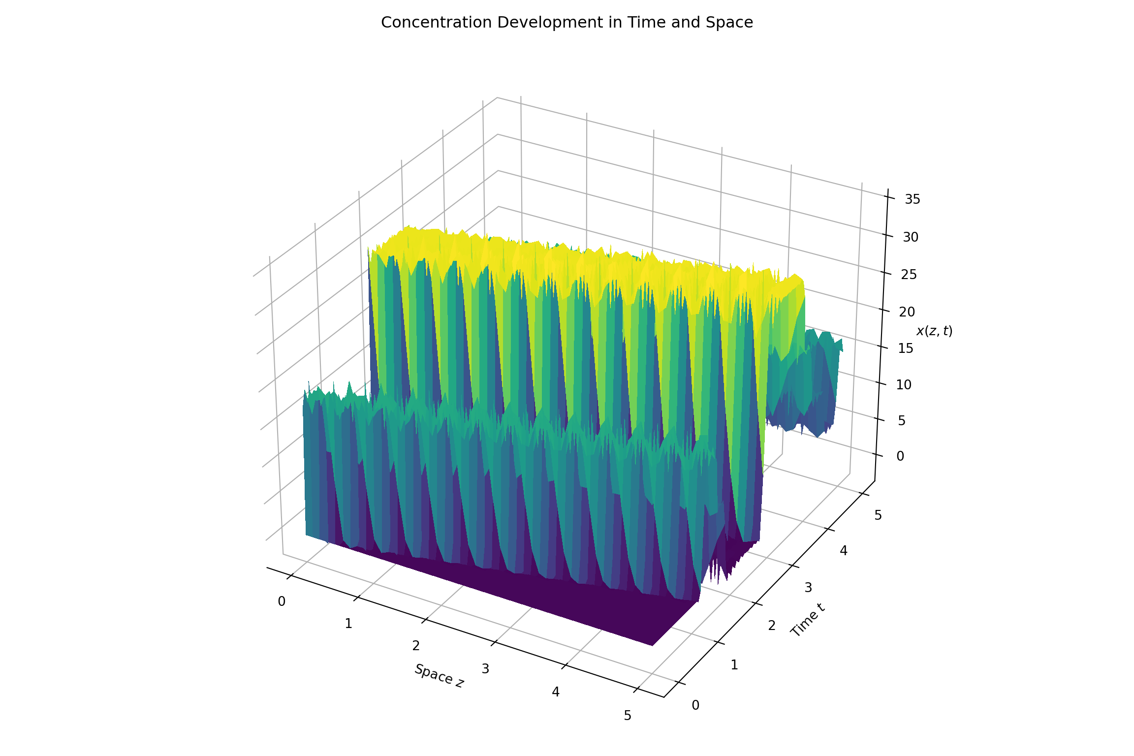
The image of the latest CI job is not available. This is a fallback image. Debug:
Path: ackrep_data/system_models/linear_transport_system View on GitHub
Type: system_model
Short Description: PDE modeling the concentration of a substance flowing in a liquid with constant speed
Created: 01.08.2022
Compatible Environment: default_conda_environment (Key: CDAMA)
Source Code [ / ] simulation.py
import numpy as np
import pyinduct as pi
import pyqtgraph as pg
import system_model
from scipy.integrate import solve_ivp
from ackrep_core import ResultContainer
from ackrep_core.system_model_management import save_plot_in_dir
import matplotlib.pyplot as plt
import matplotlib
import os
from ipydex import IPS
# link to documentation with examples: https://ackrep-doc.readthedocs.io/en/latest/devdoc/contributing_data.html
def simulate():
"""
simulate the system model with scipy.integrate.solve_ivp
:return: result of solve_ivp, might contains input function
"""
model = system_model.Model()
print(">>> derive initial conditions")
q0 = pi.core.project_on_bases(model.initial_states, model.canonical_equations)
print(">>> perform time step integration")
sim_domain, q = pi.simulate_state_space(model.state_space_form, q0, model.temp_domain, settings=None)
print(">>> perform postprocessing")
eval_data = pi.get_sim_results(
sim_domain, model.spatial_domains, q, model.state_space_form, derivative_orders=model.derivative_orders
)
evald_x = pi.evaluate_approximation(model.func_label, q, sim_domain, model.spat_domain, name="x(z,t)")
pi.tear_down(labels=(model.func_label,))
sim = ResultContainer()
sim.u = model.u.get_results(eval_data[0].input_data[0]).flatten()
sim.eval_data = eval_data
sim.evald_x = evald_x
save_plot(sim)
return sim
def save_plot(simulation_data):
"""
plot your data and save the plot
access to data via: simulation_data.t array of time values
simulation_data.y array of data components
simulation_data.uu array of input values
:param simulation_data: simulation_data of system_model
:return: None
"""
# Note: plotting in pyinduct is usually done with pyqtgraph which causes issues during CI.
# This is why the plotting part doesnt look as clean.
# Pyinduct has its own plotting methods, feel free to use them in your own implementation.
matplotlib.use("Agg")
# imput data
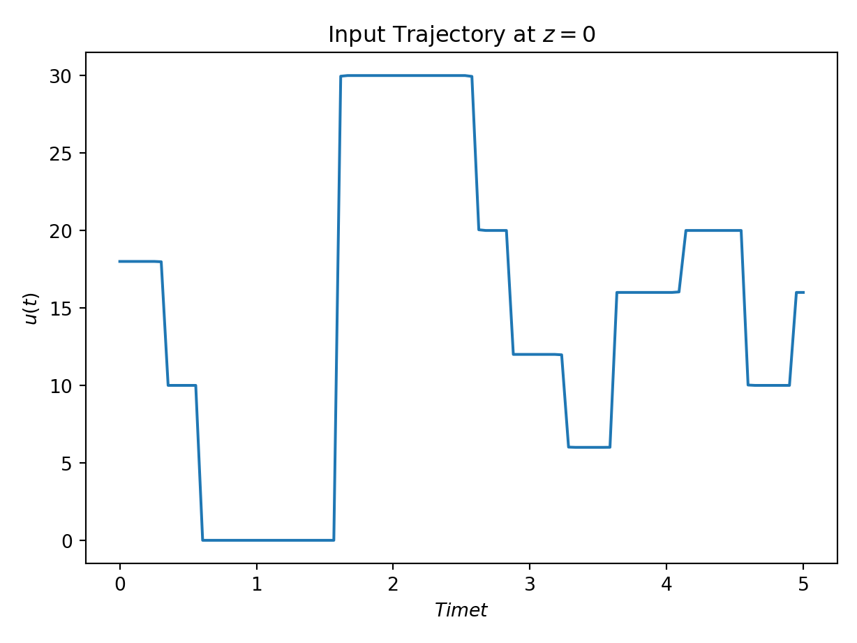
win0 = plt.plot(np.array(simulation_data.eval_data[0].input_data[0]).flatten(), simulation_data.u)
plt.title("Input Trajectory at $z=0$")
plt.xlabel("Time $t$")
plt.ylabel("$u(t)$")
plt.grid()
plt.tight_layout()
save_plot_in_dir("plot_1.png")
win1 = pi.surface_plot(simulation_data.evald_x, zlabel="$x(z,t)$")
plt.title("Concentration Development in Time and Space")
plt.ylabel("Time $t$")
plt.xlabel("Space $z$")
plt.tight_layout()
save_plot_in_dir("plot_2.png")
# Animation, try it yourself!
# win1 = pi.PgAnimatedPlot(simulation_data.eval_data,
# title=simulation_data.eval_data[0].name,
# save_pics=False,
# labels=dict(left='x(z,t)', bottom='z'))
# pi.show()
def evaluate_simulation(simulation_data):
"""
assert that the simulation results are as expected
:param simulation_data: simulation_data of system_model
:return:
"""
expected_final_state = np.array(
[
15.9121583,
16.09994978,
15.96335188,
13.08588575,
10.13711019,
9.6499634,
10.67303024,
9.56644162,
9.6876343,
10.81433698,
9.47145433,
9.78543658,
10.2484261,
10.46145942,
10.07941574,
8.39027042,
10.62520391,
15.32583395,
18.08964,
20.24542305,
20.23232229,
19.50687173,
20.68567787,
19.68595808,
19.74016142,
20.61134939,
19.46946518,
20.02071643,
20.34514596,
19.79538786,
20.24498947,
19.23078654,
20.35257698,
21.04011064,
19.34567931,
17.950876,
17.65966753,
15.85793459,
15.24560711,
16.65874833,
16.06310628,
16.02844423,
15.17596104,
16.30717104,
17.11405632,
15.38434346,
14.70405961,
16.91689234,
17.17063399,
15.29347108,
14.99877943,
]
)
rc = ResultContainer(score=1.0)
simulated_final_state = simulation_data.eval_data[0].output_data[-1]
rc.final_state_errors = [
simulated_final_state[i] - expected_final_state[i] for i in np.arange(0, len(simulated_final_state))
]
rc.success = np.allclose(expected_final_state, simulated_final_state, rtol=0, atol=1e-2)
return rc
import pyinduct as pi
import numpy as np
from ipydex import IPS
import scipy
import matplotlib.pyplot as plt
import pyqtgraph as pg

sys_name = "transport_system"


# --- modelling ---
v = 4
l = 5
T = 5
spat_bounds = (0, l)
spat_domain = pi.Domain(bounds=spat_bounds, num=51)
temp_domain = pi.Domain(bounds=(0, T), num=100)

init_x = pi.Function(lambda z: 0, domain=spat_bounds)

init_funcs = pi.LagrangeFirstOrder.cure_interval(spat_domain)
func_label = "init_funcs"
pi.register_base(func_label, init_funcs)
# inpuc function
u = pi.SimulationInputSum(
    [
        pi.SignalGenerator("square", np.array(temp_domain), frequency=0.1, scale=1, offset=1, phase_shift=1),
        pi.SignalGenerator("square", np.array(temp_domain), frequency=0.2, scale=2, offset=2, phase_shift=2),
        pi.SignalGenerator("square", np.array(temp_domain), frequency=0.3, scale=3, offset=3, phase_shift=3),
        pi.SignalGenerator("square", np.array(temp_domain), frequency=0.4, scale=4, offset=4, phase_shift=4),
        pi.SignalGenerator("square", np.array(temp_domain), frequency=0.5, scale=5, offset=5, phase_shift=5),
    ]
)

x = pi.FieldVariable(func_label)
phi = pi.TestFunction(func_label)

weak_form = pi.WeakFormulation(
    [
        pi.IntegralTerm(pi.Product(x.derive(temp_order=1), phi), spat_bounds),
        pi.IntegralTerm(pi.Product(x, phi.derive(1)), spat_bounds, scale=-v),
        pi.ScalarTerm(pi.Product(x(l), phi(l)), scale=v),
        pi.ScalarTerm(pi.Product(pi.Input(u), phi(0)), scale=-v),
    ],
    name=sys_name,
)

ics = pi.sanitize_input(init_x, pi.core.Function)
initial_states = {weak_form.name: ics}
spatial_domains = {weak_form.name: spat_domain}
derivative_orders = {weak_form.name: (0, 0)}

weak_forms = pi.sanitize_input([weak_form], pi.WeakFormulation)
print("simulate systems: {}".format([f.name for f in weak_forms]))

print(">>> parse weak formulations")
canonical_equations = pi.parse_weak_formulations(weak_forms)

print(">>> create state space system")
state_space_form = pi.create_state_space(canonical_equations)

# --- simulation ---

print(">>> derive initial conditions")
q0 = pi.core.project_on_bases(initial_states, canonical_equations)

print(">>> perform time step integration")
sim_domain, q = pi.simulate_state_space(state_space_form, q0, temp_domain, settings=None)

print(">>> perform postprocessing")
eval_data = pi.get_sim_results(sim_domain, spatial_domains, q, state_space_form, derivative_orders=derivative_orders)

evald_x = pi.evaluate_approximation(func_label, q, sim_domain, spat_domain, name="x(z,t)")

pi.tear_down(labels=(func_label,))


# pyqtgraph visualization
win0 = pi.surface_plot(evald_x, zlabel=evald_x.name)

# IPS()

# pyqtgraph visualization
win1 = pg.plot(
    np.array(eval_data[0].input_data[0]).flatten(),
    u.get_results(eval_data[0].input_data[0]).flatten(),
    labels=dict(left="u(t)", bottom="t"),
    pen="b",
)

plt.plot(np.array(eval_data[0].input_data[0]).flatten(), u.get_results(eval_data[0].input_data[0]).flatten())
plt.show()
# IPS()

win1.showGrid(x=False, y=True, alpha=0.5)

import pyqtgraph.exporters as exp

exporter = exp.ImageExporter(win1.plotItem)
# exporter.export("input.png")


# vis.save_2d_pg_plot(win0, 'transport_system')
# win2 = pi.PgAnimatedPlot(eval_data,
#                             title=eval_data[0].name,
#                             save_pics=True,
#                             create_video=True,
#                             labels=dict(left='x(z,t)', bottom='z'))
# pi.show()
import sympy as sp
import symbtools as st
import importlib
import sys, os
import pyinduct as pi
import numpy as np
from ipydex import IPS, activate_ips_on_exception

from ackrep_core.system_model_management import GenericModel, import_parameters


class Model:
    # Import parameter_file
    params = import_parameters()

    v = [float(i[1]) for i in params.get_default_parameters().items()][0]
    T = 5
    l = 5
    spat_bounds = (0, l)
    spat_domain = pi.Domain(bounds=spat_bounds, num=51)
    temp_domain = pi.Domain(bounds=(0, T), num=100)

    init_x = pi.Function(lambda z: 0, domain=spat_bounds)

    init_funcs = pi.LagrangeFirstOrder.cure_interval(spat_domain)
    func_label = "init_funcs"
    pi.register_base(func_label, init_funcs, overwrite=True)
    # inpuc function
    u = pi.SimulationInputSum(
        [
            pi.SignalGenerator("square", np.array(temp_domain), frequency=0.1, scale=1, offset=1, phase_shift=1),
            pi.SignalGenerator("square", np.array(temp_domain), frequency=0.2, scale=2, offset=2, phase_shift=2),
            pi.SignalGenerator("square", np.array(temp_domain), frequency=0.3, scale=3, offset=3, phase_shift=3),
            pi.SignalGenerator("square", np.array(temp_domain), frequency=0.4, scale=4, offset=4, phase_shift=4),
            pi.SignalGenerator("square", np.array(temp_domain), frequency=0.5, scale=5, offset=5, phase_shift=5),
        ]
    )

    x = pi.FieldVariable(func_label)
    phi = pi.TestFunction(func_label)

    # weak formulation is starting point for calculation (see documentation)
    weak_form = pi.WeakFormulation(
        [
            pi.IntegralTerm(pi.Product(x.derive(temp_order=1), phi), spat_bounds),
            pi.IntegralTerm(pi.Product(x, phi.derive(1)), spat_bounds, scale=-v),
            pi.ScalarTerm(pi.Product(x(l), phi(l)), scale=v),
            pi.ScalarTerm(pi.Product(pi.Input(u), phi(0)), scale=-v),
        ],
        name=params.model_name,
    )

    ics = pi.sanitize_input(init_x, pi.core.Function)
    initial_states = {weak_form.name: ics}
    spatial_domains = {weak_form.name: spat_domain}
    derivative_orders = {weak_form.name: (0, 0)}

    weak_forms = pi.sanitize_input([weak_form], pi.WeakFormulation)
    print("simulate systems: {}".format([f.name for f in weak_forms]))

    print(">>> parse weak formulations")
    canonical_equations = pi.parse_weak_formulations(weak_forms)

    print(">>> create state space system")
    state_space_form = pi.create_state_space(canonical_equations)
# -*- coding: utf-8 -*-
"""
Created on Fri Jun 11 13:51:06 2021

@author: Jonathan Rockstroh
"""
import sys
import os
import numpy as np
import sympy as sp

import tabulate as tab


# tailing "_nv" stands for "numerical value"


model_name = "Transport_System"

# CREATE SYMBOLIC PARAMETERS
pp_symb = [v] = [sp.symbols("v", real=True)]


# SYMBOLIC PARAMETER FUNCTIONS
v_sf = 4


# List of symbolic parameter functions
pp_sf = [v_sf]


# List for Substitution
pp_subs_list = []

# OPTONAL: Dictionary which defines how certain variables shall be written
# in the tabular - key: Symbolic Variable, Value: LaTeX Representation/Code
# useful for example for complex variables: {Z: r"\underline{Z}"}
latex_names = {}


# ---------- CREATE BEGIN OF LATEX TABULAR
# Define tabular Header

# DON'T CHANGE FOLLOWING ENTRIES: "Symbol", "Value"
tabular_header = ["Parameter Name", "Symbol", "Value"]

# Define column text alignments
col_alignment = ["left", "center", "center"]

# Define Entries of all columns before the Symbol-Column
# --- Entries need to be latex code
col_1 = ["velocity-constant"]

# contains all lists of the columns before the "Symbol" Column
# --- Empty list, if there are no columns before the "Symbol" Column
start_columns_list = [col_1]


# contains all lists of columns after the FIX ENTRIES
# --- Empty list, if there are no columns after the "Value" column
end_columns_list = []
Related Problems:
Extensive Material:
Download pdf
Result: Script Error.
Last Build: Checkout CI Build
Runtime: 2.3 (estimated: 15s)
Entity passed last: 2023-07-03 13:14:44
with ackrep_data commit: {'author': 'JuliusFiedler', 'branch': 'develop', 'date': '2023-07-03 13:12:35', 'message': 'fix typos and folder names', 'sha': '180d385f485e4aa0d3df6c7a716fa9d1270dc4f3'}
with ackrep_core commit: {'author': 'JuliusFiedler', 'branch': 'develop', 'date': '2023-07-03 09:44:41', 'message': 'black', 'sha': '2bde08d26afc7227546533ecd58f249d24063462'}
in environment: default_conda_environment:0.1.12
Checkout CI Build
Plot:with ackrep_data commit: {'author': 'JuliusFiedler', 'branch': 'develop', 'date': '2023-07-03 13:12:35', 'message': 'fix typos and folder names', 'sha': '180d385f485e4aa0d3df6c7a716fa9d1270dc4f3'}
with ackrep_core commit: {'author': 'JuliusFiedler', 'branch': 'develop', 'date': '2023-07-03 09:44:41', 'message': 'black', 'sha': '2bde08d26afc7227546533ecd58f249d24063462'}
in environment: default_conda_environment:0.1.12
Checkout CI Build
The image of the latest CI job is not available. This is a fallback image.
The image of the latest CI job is not available. This is a fallback image. Debug:
Checking <SystemModel (pk: 138, key: IG3GA)> "(linear transport system, 15s)"
13:02:41 - ackrep - INFO -   ... Creating exec-script ...
13:02:41 - ackrep - INFO - execscript-path: /code/ackrep/ackrep_data/execscript.py
13:02:41 - ackrep - INFO -   ... running exec-script /code/ackrep/ackrep_data/execscript.py ...
13:02:43 - ackrep - ERROR -
        The command `python /code/ackrep/ackrep_data/execscript.py` exited with returncode 1.

        stdout:

        stderr: Traceback (most recent call last):
  File "/code/ackrep/ackrep_data/execscript.py", line 35, in <module>
    import system_model
  File "/code/ackrep/ackrep_data/system_models/linear_transport_system/system_model.py", line 5, in <module>
    import pyinduct as pi
  File "/opt/conda/lib/python3.8/site-packages/pyinduct/__init__.py", line 17, in <module>
    from .eigenfunctions import *
  File "/opt/conda/lib/python3.8/site-packages/pyinduct/eigenfunctions.py", line 24, in <module>
    from .visualization import visualize_roots
  File "/opt/conda/lib/python3.8/site-packages/pyinduct/visualization.py", line 19, in <module>
    import pyqtgraph.opengl as gl
  File "/opt/conda/lib/python3.8/site-packages/pyqtgraph/opengl/__init__.py", line 1, in <module>
    from . import shaders
  File "/opt/conda/lib/python3.8/site-packages/pyqtgraph/opengl/shaders.py", line 1, in <module>
    from OpenGL.GL import *  # noqa
  File "/opt/conda/lib/python3.8/site-packages/OpenGL/GL/__init__.py", line 4, in <module>
    from OpenGL.GL.VERSION.GL_1_1 import *
  File "/opt/conda/lib/python3.8/site-packages/OpenGL/GL/VERSION/GL_1_1.py", line 14, in <module>
    from OpenGL.raw.GL.VERSION.GL_1_1 import *
  File "/opt/conda/lib/python3.8/site-packages/OpenGL/raw/GL/VERSION/GL_1_1.py", line 7, in <module>
    from OpenGL.raw.GL import _errors
  File "/opt/conda/lib/python3.8/site-packages/OpenGL/raw/GL/_errors.py", line 4, in <module>
    _error_checker = _ErrorChecker( _p, _p.GL.glGetError )
AttributeError: 'NoneType' object has no attribute 'glGetError'


Fail.