Automatic Control Knowledge Repository

#!/usr/bin/env python3
# -*- coding: utf-8 -*-
"""
problem solution for control problem: design a controller by using linear trajectory planning.
"""
try:
    import coprime_decomposition as cd  # noqa
except ImportError:
    from method_packages.coprime_decomposition import coprime_decomposition as cd

import sympy as sp
import symbtools as st
import matplotlib.pyplot as plt
import method_trajectory_planning as tp  # noqa
import control
from control import matlab
import os
from ackrep_core.system_model_management import save_plot_in_dir


class SolutionData:
    pass


def solve(problem_spec):
    s, t, T = sp.symbols("s, t, T")
    # transfer function of system
    transfer_func = problem_spec.transfer_func()
    z_func, n_func = transfer_func.expand().as_numer_denom()  # separate numerator and denominator
    z_coeffs = [float(c) for c in st.coeffs(z_func, s)]  # coefficients of numerator
    n_coeffs = [float(c) for c in st.coeffs(n_func, s)]  # coefficients of denominator

    b_0 = z_func.coeff(s, 0)
    # Boundary conditions for q and its derivative
    q_a = [problem_spec.YA[0] / b_0, 0]
    q_e = [problem_spec.YB[0] / b_0, 0]

    # generate trajectory of q(t)
    planer = tp.Trajectory_Planning(q_a, q_e, problem_spec.t0, problem_spec.tf, problem_spec.tt)
    planer.dem = n_func
    planer.num = z_func
    q_poly = planer.calc_trajectory()

    # trajectory of input and output
    u_poly, y_poly = planer.num_den_laplace(q_poly[0])

    q_func = st.expr_to_func(t, q_poly[0])
    u_func = st.expr_to_func(t, u_poly)  # desired input trajectory function
    y_func = st.expr_to_func(t, y_poly)  # desired output trajectory function

    # tracking controller
    # numerator and denominator of controller
    cd_res = cd.coprime_decomposition(z_func, n_func, problem_spec.poles)

    # open_loop k(s) * P(s)
    tf_k = (cd_res.f_func * z_func) / (cd_res.h_func * n_func)
    z_o, n_o = sp.simplify(tf_k).expand().as_numer_denom()

    # coefficients of controller
    z_coeffs_c = [float(c) for c in st.coeffs(cd_res.f_func, s)]  # coefficients of numerator
    n_coeffs_c = [float(c) for c in st.coeffs(cd_res.h_func, s)]  # coefficients of denominator

    # coefficients of open loop
    z_coeffs_o = [float(c) for c in st.coeffs(z_o, s)]
    n_coeffs_o = [float(c) for c in st.coeffs(n_o, s)]

    # In order to simulate the closed loop system with the controller,
    # the system is divided into two subsystems. one of them with the y_ref as input
    # and the other with u_ref
    close_loop_1 = control.feedback(control.tf(z_coeffs_o, n_coeffs_o))
    close_loop_2 = control.feedback(control.tf(z_coeffs, n_coeffs), control.tf(z_coeffs_c, n_coeffs_c))

    # subsystem 1 with y_ref
    y_1 = control.forced_response(close_loop_1, problem_spec.tt2, y_func(problem_spec.tt2), problem_spec.x0_1)
    # subsystem 2 with u_ref
    y_2 = control.forced_response(close_loop_2, problem_spec.tt2, u_func(problem_spec.tt2), problem_spec.x0_2)

    solution_data = SolutionData()
    solution_data.u = u_func
    solution_data.q = q_func
    solution_data.y_1 = y_1[1]
    solution_data.y_2 = y_2[1]
    solution_data.y_func = y_func

    save_plot(problem_spec, solution_data)

    return solution_data


def save_plot(problem_spec, solution_data):
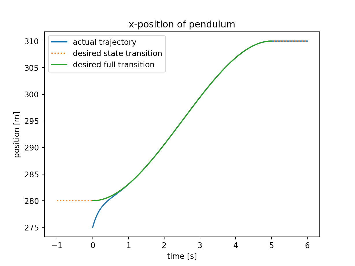
    plt.figure(1)  # simulated trajectory of CuZn-ball
    plt.plot(problem_spec.tt2, solution_data.y_1 + solution_data.y_2, label="actual trajectory")
    plt.plot(problem_spec.tt1, solution_data.y_func(problem_spec.tt1), ":", label="desired state transition")
    plt.plot(problem_spec.tt, solution_data.y_func(problem_spec.tt), label="desired full transition")
    plt.xlabel("time [s]")
    plt.ylabel("position [m]")
    plt.title("x-position of pendulum")
    plt.legend(loc=2)

    # save image
    save_plot_in_dir()