Automatic Control Knowledge Repository
You currently have javascript disabled. Some features will be unavailable. Please consider enabling javascript.Details for: "SINDy for Lotka Volterra Model"
Name: SINDy for Lotka Volterra Model
(Key: QWRHA)
Path: ackrep_data/problem_solutions/PySINDy_identify_volterra View on GitHub
Type: problem_solution
Short Description: reconstructs lotka volterra equations from data using PySINDy
Created: 2022-08-05
Compatible Environment: default_conda_environment (Key: CDAMA)
Source Code [ / ] solution.py
Solved Problems: SINDy for Lotka Volterra Model |
Used Methods:
Result: Success.
Last Build: Checkout CI Build
Runtime: 4.8 (estimated: 15s)
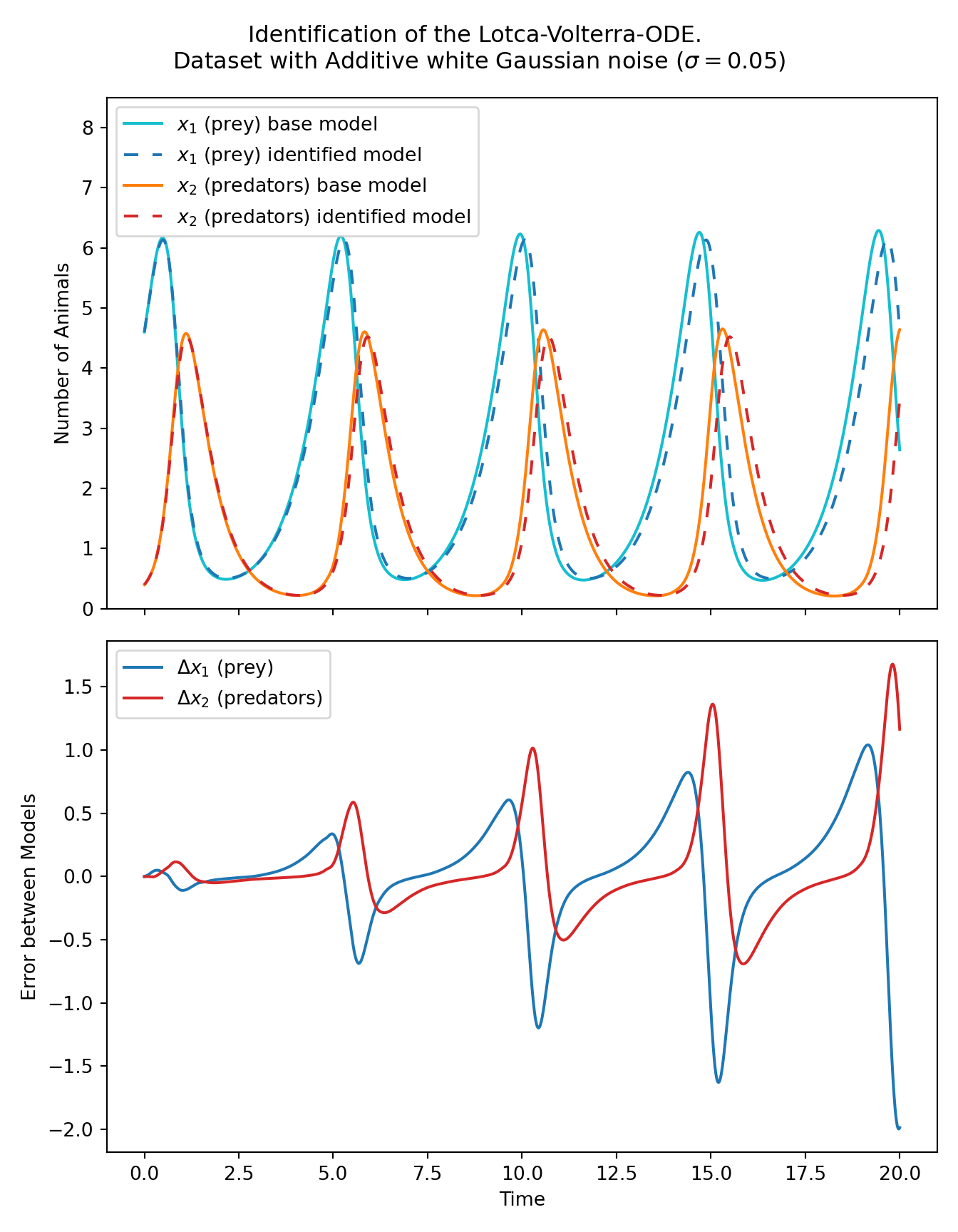
Plot:

The image of the latest CI job is not available. This is a fallback image.
Path: ackrep_data/problem_solutions/PySINDy_identify_volterra View on GitHub
Type: problem_solution
Short Description: reconstructs lotka volterra equations from data using PySINDy
Created: 2022-08-05
Compatible Environment: default_conda_environment (Key: CDAMA)
Source Code [ / ] solution.py
#!/usr/bin/env python3
# -*- coding: utf-8 -*-

import matplotlib.pyplot as plt
import symbtools as st
from scipy.integrate import solve_ivp
import sympy as sp
import os
import numpy as np
from ackrep_core.system_model_management import save_plot_in_dir
import pysindy as ps
from ipydex import IPS


class SolutionData:
    pass


def solve(problem_spec):

    # identify the model
    differentiation_method = ps.FiniteDifference(order=2)
    feature_library = ps.PolynomialLibrary(degree=2)
    optimizer = ps.STLSQ(threshold=0.2)
    sindy_model = ps.SINDy(
        differentiation_method=differentiation_method,
        feature_library=feature_library,
        optimizer=optimizer,
        feature_names=["x1", "y2"],
    )
    # add some noise to training data
    xx_train_clean = problem_spec.xx_train.y.transpose()
    np.random.seed(1)
    xx_train_noisy = xx_train_clean + np.random.normal(scale=0.05, size=xx_train_clean.shape)

    sindy_model.fit(xx_train_noisy, t=0.002)
    print("Identified Equations:")
    sindy_model.print()

    # simulate identified model
    xx0_test = problem_spec.xx0_test
    tt_test = problem_spec.tt_test
    xx_test = problem_spec.xx_test.y.transpose()
    xx_sim = sindy_model.simulate(xx0_test, tt_test)

    # Evolve the new initial condition in time with the SINDy model
    fig, axs = plt.subplots(2, 1, sharex=True, figsize=(7, 9))
    fig.suptitle(
        "Identification of the Lotca-Volterra-ODE. \nDataset with Additive white Gaussian noise $(\sigma=0.05)$"
    )
    axs[0].plot(tt_test, xx_test[:, 0], color="tab:cyan", label="$x_1$ (prey) base model")
    axs[0].plot(tt_test, xx_sim[:, 0], color="tab:blue", linestyle=(0, (5, 5)), label="$x_1$ (prey) identified model")
    axs[0].plot(tt_test, xx_test[:, 1], color="tab:orange", label="$x_2$ (predators) base model")
    axs[0].plot(
        tt_test, xx_sim[:, 1], color="tab:red", linestyle=(0, (5, 5)), label="$x_2$ (predators) identified model"
    )
    axs[0].legend()
    axs[0].set(ylabel="Number of Animals", ylim=(0, 8.5))

    axs[1].plot(tt_test, xx_test[:, 0] - xx_sim[:, 0], color="tab:blue", label="$\Delta x_1$ (prey)")
    axs[1].plot(tt_test, xx_test[:, 1] - xx_sim[:, 1], color="tab:red", label="$\Delta x_2$ (predators)")
    axs[1].legend()
    axs[1].set(xlabel="Time", ylabel="Error between Models")

    solution_data = SolutionData()
    solution_data.xx_sim = xx_sim.transpose()

    plt.tight_layout()
    save_plot_in_dir()

    return solution_data
Solved Problems: SINDy for Lotka Volterra Model |
Used Methods:
Result: Success.
Last Build: Checkout CI Build
Runtime: 4.8 (estimated: 15s)
Plot:

The image of the latest CI job is not available. This is a fallback image.