Automatic Control Knowledge Repository
You currently have javascript disabled. Some features will be unavailable. Please consider enabling javascript.Details for: "kapitza's pendulum"
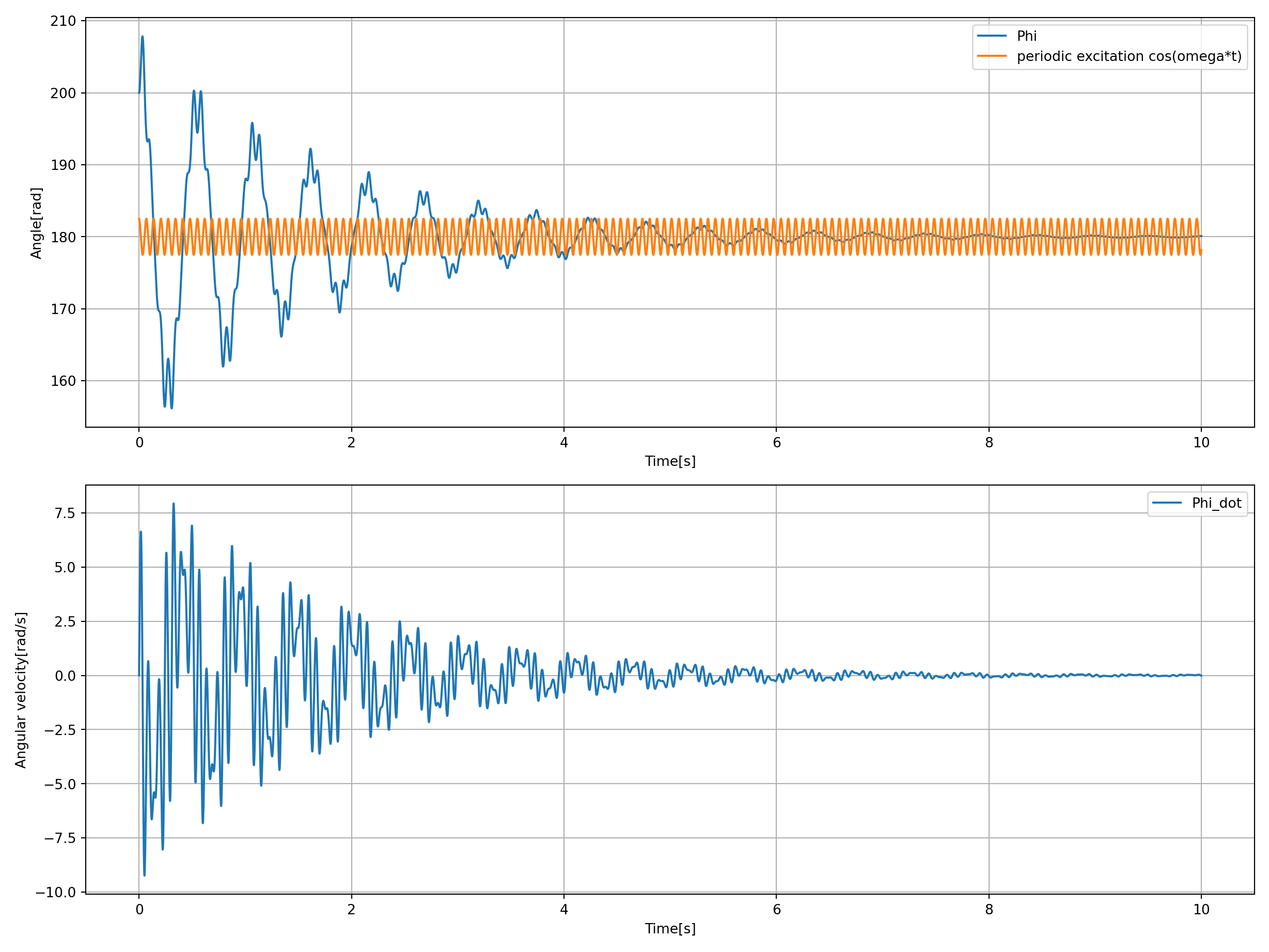
Name: kapitza's pendulum
(Key: U6B7N)
Path: ackrep_data/system_models/kapitzas_pendulum_system View on GitHub
Type: system_model
Short Description: nonlinear physical system, rigid pendulum in which the pivot point vibrates in a vertical direction
Created: 2022-04-21
Compatible Environment: default_conda_environment (Key: CDAMA)
Source Code [ / ] simulation.py
Related Problems:
Extensive Material:
Download pdf
Result: Success.
Last Build: Checkout CI Build
Runtime: 3.7 (estimated: 10s)
Plot:
The image of the latest CI job is not available. This is a fallback image.
Path: ackrep_data/system_models/kapitzas_pendulum_system View on GitHub
Type: system_model
Short Description: nonlinear physical system, rigid pendulum in which the pivot point vibrates in a vertical direction
Created: 2022-04-21
Compatible Environment: default_conda_environment (Key: CDAMA)
Source Code [ / ] simulation.py
# -*- coding: utf-8 -*-
"""
Created on Mon Jun  7 19:06:37 2021

@author: Rocky
"""

import numpy as np
import system_model
from scipy.integrate import solve_ivp

from ackrep_core import ResultContainer
from ackrep_core.system_model_management import save_plot_in_dir
import matplotlib.pyplot as plt
import os


def simulate():
    model = system_model.Model()

    rhs_xx_pp_symb = model.get_rhs_symbolic()
    print("Computational Equations:\n")
    for i, eq in enumerate(rhs_xx_pp_symb):
        print(f"dot_x{i+1} =", eq)

    rhs = model.get_rhs_func()

    # Initial State values
    xx0 = [200 / 360 * 2 * np.pi, 0]

    t_end = 10
    tt = times = np.linspace(0, t_end, 10000)
    sim = solve_ivp(rhs, (0, t_end), xx0, t_eval=tt)

    uu = model.uu_func(sim.t, xx0)[0] * 0.005 + 180
    sim.uu = uu

    save_plot(sim)

    return sim


def save_plot(sim):

    # create figure + 2x2 axes array
    fig1, axs = plt.subplots(nrows=2, ncols=1, figsize=(12.8, 9.6))

    # print in axes top left
    axs[0].plot(sim.t, np.real(sim.y[0] * 360 / (2 * np.pi)), label=r"$\varphi$")

    axs[0].plot(sim.t, list(sim.uu), label=r"periodic excitation $\cos(\omega*t)$")
    axs[0].set_ylabel("Angle [rad]")  # y-label
    axs[0].grid()
    axs[0].legend()

    # print in axes top right
    axs[1].plot(sim.t, np.real(sim.y[1]))
    axs[1].set_ylabel("Angular velocity [rad/s]")  # y-label
    axs[1].set_xlabel("Time [s]")  # x-Label
    axs[1].grid()

    plt.tight_layout()

    ## static
    save_plot_in_dir()


def evaluate_simulation(simulation_data):
    """

    :param simulation_data: simulation_data of system_model
    :return:
    """

    expected_final_state = [3.1432908256013783, -0.014961262100684384]

    rc = ResultContainer(score=1.0)
    simulated_final_state = simulation_data.y[:, -1]
    rc.final_state_errors = [
        simulated_final_state[i] - expected_final_state[i] for i in np.arange(0, len(simulated_final_state))
    ]
    rc.success = np.allclose(expected_final_state, simulated_final_state, rtol=0, atol=1e-2)

    return rc
# -*- coding: utf-8 -*-
"""
Created on Wed Jun  9 13:33:34 2021

@author: Jonathan Rockstroh
"""

import sympy as sp
import symbtools as st
import importlib
import sys, os
from ipydex import IPS, activate_ips_on_exception  # for debugging only

from ackrep_core.system_model_management import GenericModel, import_parameters

# Import parameter_file
params = import_parameters()


class Model(GenericModel):
    def initialize(self):
        """
        this function is called by the constructor of GenericModel

        :return: None
        """

        # Define number of inputs
        self.u_dim = 1

        # Set "sys_dim" to constant value, if system dimension is constant
        self.sys_dim = 2

        # check existance of params file -> if not: System is defined to hasn't
        # parameters
        self.has_params = True
        self.params = params

    # ----------- SET DEFAULT INPUT FUNCTION ---------- #
    # --------------- Only for non-autonomous Systems
    # --------------- MODEL DEPENDENT

    def uu_default_func(self):
        """
        :return:(function with 2 args - t, xx_nv) default input function
        """
        a, omega = self.pp_symb[2], self.pp_symb[3]
        u_sp = self.pp_dict[a] * sp.sin(self.pp_dict[omega] * self.t_symb - sp.pi / 2)
        du_dtt_sp = u_sp.diff(self.t_symb, 2)
        du_dtt_sp = du_dtt_sp.subs(self.pp_subs_list)
        du_dtt_func = st.expr_to_func(self.t_symb, du_dtt_sp)

        def uu_rhs(t, xx_nv):
            du_dtt_nv = du_dtt_func(t)
            return [du_dtt_nv]

        return uu_rhs

    # ----------- SYMBOLIC RHS FUNCTION ---------- #
    # --------------- MODEL DEPENDENT

    def get_rhs_symbolic(self):
        """
        :return:(matrix) symbolic rhs-functions
        """
        if self.dxx_dt_symb is not None:
            return self.dxx_dt_symb
        x1, x2 = self.xx_symb
        l, g, a, omega, gamma = self.pp_symb
        # u0 = input force
        u0 = self.uu_symb[0]
        # create symbolic rhs functions
        dx1_dt = x2
        dx2_dt = -2 * gamma * x2 - (g / l + 1 / l * u0) * sp.sin(x1)

        # put rhs functions into a vector
        self.dxx_dt_symb = sp.Matrix([dx1_dt, dx2_dt])

        return self.dxx_dt_symb
# -*- coding: utf-8 -*-
"""
Created on Fri Jun 11 13:51:06 2021

@author: Jonathan Rockstroh
"""
import sys
import os
import numpy as np
import sympy as sp

import tabulate as tab


model_name = "Kapitzas_Pendulum"

# --------- CREATE SYMBOLIC PARAMETERS
pp_symb = [l, g, a, omega, gamma] = sp.symbols("l, g, a, omega, gamma", real=True)

# -------- CREATE AUXILIARY SYMBOLIC PARAMETERS
# (parameters, which shall not be numerical represented in the parameter tabular)
omega_0 = sp.Symbol("omega_0")

# --------- SYMBOLIC PARAMETER FUNCTIONS
# ------------ parameter values can be constant/fixed values OR
# ------------ set in relation to other parameters (for example: a = 2*b)
l_sf = 30 / 100
g_sf = 9.81
a_sf = 1 / 5 * l
omega_sf = 16 * omega_0
gamma_sf = 0.1 * omega_0

# List of symbolic parameter functions
pp_sf = [l_sf, g_sf, a_sf, omega_sf, gamma_sf]

# Set numerical values of auxiliary parameters
omega_0_nv = np.sqrt(g_sf / l_sf)

# List for Substitution
# -- Entries are tuples like: (independent symbolic parameter, numerical value)
pp_subs_list = [(l, l_sf), (omega_0, omega_0_nv)]

# OPTONAL: Dictionary which defines how certain variables shall be written
# in the tabular - key: Symbolic Variable, Value: LaTeX Representation/Code
# useful for example for complex variables: {Z: r"\underline{Z}"}
latex_names = {}


# ---------- CREATE BEGIN OF LATEX TABULAR

# Define tabular Header
# DON'T CHANGE FOLLOWING ENTRIES: "Symbol", "Value"
tabular_header = ["Parameter Name", "Symbol", "Value", "Unit"]

# Define column text alignments
col_alignment = ["left", "center", "left", "center"]

# Define Entries of all columns before the Symbol-Column
# --- Entries need to be latex code

col_1 = [
    "Pendulum length",
    "acceleration due to gravitation",
    "Amplitude of Oscillation",
    "Frequency of Oscillation",
    "Dampening Factor",
]
# contains all lists of the columns before the "Symbol" Column
# --- Empty list, if there are no columns before the "Symbol" Column
start_columns_list = [col_1]

# Define Entries of the columns after the Value-Column
# --- Entries need to be latex code
col_4 = ["cm", r"$\frac{m}{s^2}$", "cm", "Hz", "Hz"]
# contains all lists of columns after the FIX ENTRIES
# --- Empty list, if there are no columns after the "Value" column
end_columns_list = [col_4]
Related Problems:
Extensive Material:
Download pdf
Result: Success.
Last Build: Checkout CI Build
Runtime: 3.7 (estimated: 10s)
Plot:
The image of the latest CI job is not available. This is a fallback image.