Automatic Control Knowledge Repository
You currently have javascript disabled. Some features will be unavailable. Please consider enabling javascript.Details for: "modular multilevel converter (MMC)"
Name: modular multilevel converter (MMC)
(Key: YHS5B)
Path: ackrep_data/system_models/mmc_system View on GitHub
Type: system_model
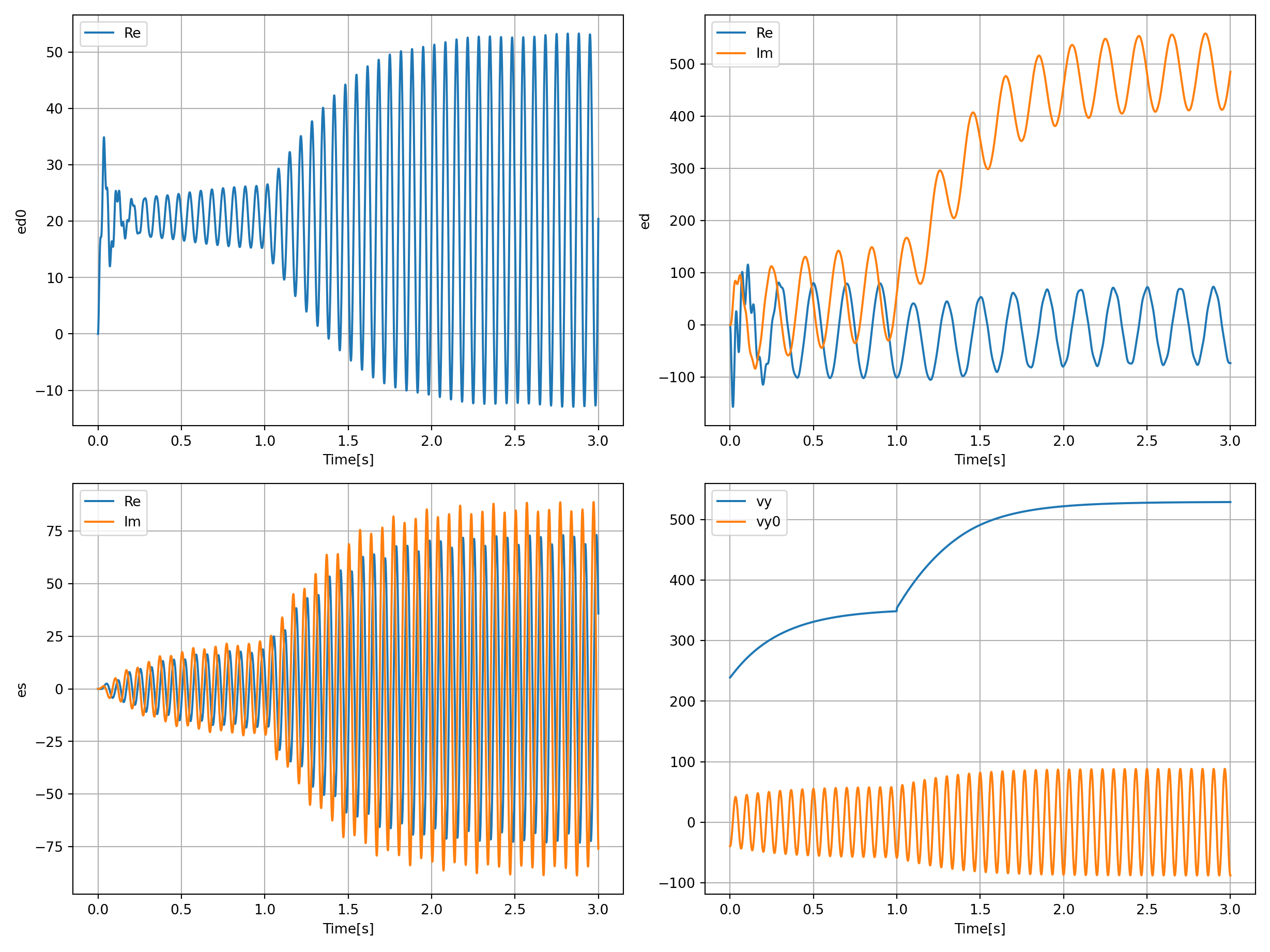
Short Description: MMC with 3 phases, 1 Submodule per Arm and output to grid. Used to generate multilevel Voltages
Created: 2022-05-09
Compatible Environment: default_conda_environment (Key: CDAMA)
Source Code [ / ] simulation.py
Related Problems:
Extensive Material:
Download pdf
Result: Success.
Last Build: Checkout CI Build
Runtime: 39.6 (estimated: 50s)
Plot:
The image of the latest CI job is not available. This is a fallback image.
Path: ackrep_data/system_models/mmc_system View on GitHub
Type: system_model
Short Description: MMC with 3 phases, 1 Submodule per Arm and output to grid. Used to generate multilevel Voltages
Created: 2022-05-09
Compatible Environment: default_conda_environment (Key: CDAMA)
Source Code [ / ] simulation.py
import numpy as np
import system_model
from scipy.integrate import solve_ivp

from ackrep_core import ResultContainer
from ackrep_core.system_model_management import save_plot_in_dir
import matplotlib.pyplot as plt
import os

import time
from ipydex import IPS, activate_ips_on_exception

activate_ips_on_exception()


def simulate():
    model = system_model.Model()

    rhs_xx_pp_symb = model.get_rhs_symbolic()
    print("Computational Equations:\n")
    for i, eq in enumerate(rhs_xx_pp_symb):
        print(f"dot_x{i+1} =", eq)

    rhs = model.get_rhs_func()

    # --------------------------------------------------------------------

    xx0 = [0, 0, 0 + 0j, 0 + 0j, 0 + 0j, 0, 0 + 0j, 0]
    t_end = 3
    tt = np.linspace(0, t_end, 3000)
    # use model class rhs
    sol = solve_ivp(rhs, (0, t_end), xx0, t_eval=tt)

    i = 0
    n_rows = len(sol.t)
    n_cols = 4
    uu = np.zeros((n_rows, n_cols))

    while i < len(sol.t):
        uu[i, :] = model.uu_func(sol.t[i], sol.y[:, i])
        i = i + 1

    sol.uu = uu

    # --------------------------------------------------------------------

    save_plot(sol)

    return sol


def save_plot(sol):

    # --------------------------------------------------------------------

    # create figure + 2x2 axes array
    fig1, axs = plt.subplots(nrows=2, ncols=2, figsize=(12.8, 9.6))

    # print in axes top left
    axs[0, 0].plot(sol.t, np.real(sol.y[1]), label="Re")
    axs[0, 0].set_ylabel("ed0")  # y-label
    axs[0, 0].set_xlabel("Time [s]")  # x-Label
    axs[0, 0].grid()
    axs[0, 0].legend()

    # print in axes top right
    axs[1, 0].plot(sol.t, np.real(sol.y[2]), label="Re")
    axs[1, 0].plot(sol.t, np.imag(sol.y[2]), label="Im")
    axs[1, 0].set_ylabel("es")  # y-label
    axs[1, 0].set_xlabel("Time [s]")  # x-Label
    axs[1, 0].grid()
    axs[1, 0].legend()

    # print in axes bottom left
    axs[0, 1].plot(sol.t, np.real(sol.y[3]), label="Re")
    axs[0, 1].plot(sol.t, np.imag(sol.y[3]), label="Im")
    axs[0, 1].set_ylabel("ed")  # y-label
    axs[0, 1].set_xlabel("Time [s]")  # x-Label
    axs[0, 1].grid()
    axs[0, 1].legend()

    # print in axes bottom right
    axs[1, 1].plot(sol.t, sol.uu[:, 0], label="vy")
    axs[1, 1].plot(sol.t, sol.uu[:, 1], label="vy0")
    axs[1, 1].set_ylabel("")  # y-label
    axs[1, 1].set_xlabel("Time [s]")  # x-Label
    axs[1, 1].grid()
    axs[1, 1].legend()

    # adjust subplot positioning and show the figure
    fig1.subplots_adjust(hspace=0.5)
    # fig1.show()

    # --------------------------------------------------------------------

    plt.tight_layout()

    save_plot_in_dir()


def evaluate_simulation(simulation_data):
    """
    :param simulation_data: simulation_data of system_model
    :return:
    """
    # --------------------------------------------------------------------
    # fill in final states of simulation to check your model
    # simulation_data.y[i][-1]
    expected_final_state = [
        (55.43841456212572 + 0j),
        (20.413747733428224 + 0j),
        (35.79509623855708 - 75.96575244375583j),
        (-72.91879818170683 + 485.1484950343515j),
        0j,
        (17.557881788491308 + 0j),
        (9.991045345136369 - 3.6215387749437133j),
        (94.24777960769383 + 0j),
    ]

    # --------------------------------------------------------------------

    rc = ResultContainer(score=1.0)
    simulated_final_state = simulation_data.y[:, -1]
    rc.final_state_errors = [
        simulated_final_state[i] - expected_final_state[i] for i in np.arange(0, len(simulated_final_state))
    ]
    rc.success = np.allclose(expected_final_state, simulated_final_state, rtol=0, atol=1e-2)

    return rc
import sympy as sp
import symbtools as st
import importlib
from sympy import I
import numpy as np
import sys, os
from ipydex import IPS, activate_ips_on_exception  # for debugging only

from ackrep_core.system_model_management import GenericModel, import_parameters

# Import parameter_file
params = import_parameters()


class Model(GenericModel):
    def initialize(self):
        """
        this function is called by the constructor of GenericModel

        :return: None
        """

        # Define number of inputs -- MODEL DEPENDENT
        self.u_dim = 4

        # Set "sys_dim" to constant value, if system dimension is constant
        # else set "sys_dim" to x_dim -- MODEL DEPENDENT
        self.sys_dim = 8

        # check existance of params file
        self.has_params = True
        self.params = params

    # ----------- SET DEFAULT INPUT FUNCTION ---------- #
    # --------------- Only for non-autonomous Systems
    # --------------- MODEL DEPENDENT

    def uu_default_func(self):
        """

        :return: (function with 2 args - t, xx_nv) default input function
        """

        vdc, vg, omega, Lz, Mz, R, L = list(self.pp_dict.values())
        Ind_sum = Mz + Lz

        def uu_rhs(t, xx_nv):

            """
            :param t:(scalar or vector) Time
            :param xx_nv: (vector or array of vectors) state vector with
                                                    numerical values at time t
            :return: [vy, vy0, vx, vx0]

            """

            es0, ed0, es, ed, iss, iss0, i, theta = xx_nv

            # Define Input Functions
            Kp = 5
            # define reference trajectory for i
            T_dur = 1.5
            tau = t / T_dur
            i_max = 10

            i_ref = 10
            dt_i_ref = 0

            if tau < 1:
                i_ref = 4 + (i_max - 4) * np.sin(0.5 * tau * np.pi) * np.sin(0.5 * tau * np.pi)
                dt_i_ref = np.pi / T_dur * np.sin(0.5 * tau * np.pi) * np.cos(0.5 * tau * np.pi)
            if t < 1:
                i_ref = 4
                dt_i_ref = 0

            vy = vg + (R + 1j * omega * L) * i + 1 * (i_ref - i) + L * dt_i_ref
            vy = complex(vy)

            vy0 = -1 / 6 * np.absolute(vy) * np.real(np.exp(3 * 1j * (theta + np.angle(vy))))

            vx = 1j * omega * Ind_sum * iss - Kp * iss  # p- controller to get iss

            # define reference trajectory of es0
            T_dur = 0.5  # duration of es0 ref_traj
            tau = t / T_dur
            # es0_max = 68
            # es0_ref = sp.Piecewise((0, tau < 0), (es0_max *sp.sin( tau*sp.pi/2)  \
            #                        *sp.sin( tau*sp.pi/2), tau < 1), (es0_max, True) )
            es0_ref = 56
            # derive iss0 ref trajectory
            iss0_ref = 1 / vdc * np.real(i * np.conjugate(vy)) + Kp * (es0_ref - es0)

            # p-controller for vx0
            vx0 = Kp * (iss0_ref - iss0)

            return [np.real(vy), vy0, vx, vx0]

        return uu_rhs

    # ----------- SYMBOLIC RHS FUNCTION ---------- #
    # --------------- MODEL DEPENDENT

    def get_rhs_symbolic(self):
        """
        :return:(matrix) symbolic rhs-functions
        """
        if self.dxx_dt_symb is not None:
            return self.dxx_dt_symb

        es0, ed0, es, ed, iss, iss0, i, theta = self.xx_symb
        vdc, vg, omega, Lz, Mz, R, L = self.pp_symb
        # u0 = input force
        vy0, vy, vx0, vx = self.uu_symb

        # Auxiliary variables
        Ind_sum = Lz + Mz
        vydelta = vy - Mz * (I * omega * i + 1 / L * (vy - (R + I * omega * L) * i - vg))

        # create symbolic rhs functions
        des0_dt = vdc * iss0 - sp.re(i * sp.conjugate(vy))

        ded0_dt = -2 * vy0 * iss0 - sp.re(sp.conjugate(iss) * vydelta)

        des_dt = vdc * iss - sp.exp(-3 * I * theta) * sp.conjugate(vy) * sp.conjugate(i) - 2 * i * vy0 - I * omega * es

        ded_dt = (
            vdc * i
            - sp.exp(-3 * I * theta) * sp.conjugate(iss) * sp.conjugate(vydelta)
            - 2 * iss * vy0
            - 2 * iss0 * vydelta
            - I * omega * ed
        )

        diss_dt = 1 / Ind_sum * (vx - I * omega * Ind_sum * iss)

        diss0_dt = vx0 / Ind_sum

        di_dt = 1 / L * (vy - (R + I * omega * L) * i - vg)

        dtheta_dt = 2 * sp.pi / 360 * omega

        # put rhs functions into a vector
        self.dxx_dt_symb = sp.Matrix([des0_dt, ded0_dt, des_dt, ded_dt, diss_dt, diss0_dt, di_dt, dtheta_dt])

        return self.dxx_dt_symb

    # ----------- NUMERIC RHS FUNCTION ---------- #
    # -------------- written sepeeratly cause it seems like that lambdify can't
    # -------------- handle complex values in a proper way

    def get_rhs_func(self):
        """
        Creates an executable function of the model which uses:
            - the current parameter values
            - the current input function

        To evaluate the effect of a changed parameter set a new rhs_func needs
        to be created with this method.

        :return:(function) rhs function for numerical solver like
                            scipy.solve_ivp
        """

        # create rhs function
        def rhs(t, xx_nv):
            """
            :param t:(tuple or list) Time
            :param xx_nv:(self.n-dim vector) numerical state vector
            :return:(self.n-dim vector) first time derivative of state vector
            """
            uu_nv = self.uu_func(t, xx_nv)
            vy, vy0, vx, vx0 = uu_nv
            es0, ed0, es, ed, iss, iss0, i, theta = xx_nv
            vdc, vg, omega, Lz, Mz, R, L = list(self.pp_dict.values())
            Ind_sum = Mz + Lz
            # = vy-Mz(j*omega*i-dt_i)
            vydelta = vy - Mz * (1j * omega * i + 1 / L * (vy - (R + 1j * omega * L) * i - vg))

            dt_es0 = vdc * iss0 - np.real(i * np.conjugate(vy))
            dt_ed0 = -2 * vy0 * iss0 - np.real(np.conjugate(iss) * vydelta)

            dt_es = (
                vdc * iss - np.exp(-3 * 1j * theta) * np.conjugate(vy) * np.conjugate(i) - 2 * i * vy0 - 1j * omega * es
            )

            dt_ed = (
                vdc * i
                - np.exp(-3 * 1j * theta) * np.conjugate(iss) * np.conjugate(vydelta)
                - 2 * iss * vy0
                - 2 * iss0 * vydelta
                - 1j * omega * ed
            )

            dt_iss = 1 / Ind_sum * (vx - 1j * omega * Ind_sum * iss)
            dt_iss0 = vx0 / Ind_sum
            dt_i = 1 / L * (vy - (R + 1j * omega * L) * i - vg)
            dt_theta = omega

            dxx_dt_nv = [dt_es0, dt_ed0, dt_es, dt_ed, dt_iss, dt_iss0, dt_i, dt_theta]

            return dxx_dt_nv

        return rhs
import sys
import os
import numpy as np
import sympy as sp

import tabulate as tab


# tailing "_nv" stands for "numerical value"

model_name = "MMC"

# --------- CREATE SYMBOLIC PARAMETERS
pp_symb = [vdc, vg, omega, Lz, Mz, R, L] = sp.symbols("v_DC, v_g, omega, L_z, M_z, R, L", real=True)

# -------- CREATE AUXILIARY SYMBOLIC PARAMETERS
# (parameters, which shall not numerical represented in the parameter tabular)

# --------- SYMBOLIC PARAMETER FUNCTIONS
# ------------ parameter values can be constant/fixed values OR
# ------------ set in relation to other parameters (for example: a = 2*b)
# ------------ useful for a clean looking parameter table in the Documentation

# Due to performance of the simulation the parameters Lz, Mz and L are choosen to be scaled with 1/10

vdc_sf = 300
vg_sf = 235
omega_sf = 2 * sp.pi * 5
Lz_sf = 1.5 / 10
Mz_sf = 0.94 / 10
R_sf = 26
L_sf = 3 / 10
# List of symbolic parameter functions
pp_sf = [vdc_sf, vg_sf, omega_sf, Lz_sf, Mz_sf, R_sf, L_sf]

# Set numerical values of auxiliary parameters

# List for Substitution
# -- Entries are tuples like: (independent symbolic parameter, numerical value)
pp_subs_list = []

# OPTONAL: Dictionary which defines how certain variables shall be written
# in the tabular - key: Symbolic Variable, Value: LaTeX Representation/Code
# useful for example for complex variables: {Z: r"\underline{Z}"}
latex_names = {}

# ---------- CREATE BEGIN OF LATEX TABULAR
# Define tabular Header

# DON'T CHANGE FOLLOWING ENTRIES: "Symbol", "Value"
tabular_header = ["Parameter Name", "Symbol", "Value", "Unit"]

# Define column text alignments
col_alignment = ["left", "center", "left", "center"]

# Define Entries of all columns before the Symbol-Column
# --- Entries need to be latex code

col_1 = [
    "DC voltage",
    "grid voltage",
    "angular speed",
    "arm inductance",
    "mutual inductance",
    "load resistance",
    "load inductance",
]
# contains all lists of the columns before the "Symbol" Column
# --- Empty list, if there are no columns before the "Symbol" Column
start_columns_list = [col_1]

# Define Entries of the columns after the Value-Column
# --- Entries need to be latex code
col_4 = ["V", "V", "Hz", "mH", "mH", r"$\Omega$", "mH"]
# contains all lists of columns after the FIX ENTRIES
# --- Empty list, if there are no columns after the "Value" column
end_columns_list = [col_4]
Related Problems:
Extensive Material:
Download pdf
Result: Success.
Last Build: Checkout CI Build
Runtime: 39.6 (estimated: 50s)
Plot:
The image of the latest CI job is not available. This is a fallback image.