Automatic Control Knowledge Repository

import numpy as np
import pyinduct as pi
import pyqtgraph as pg
import system_model
from scipy.integrate import solve_ivp

from ackrep_core import ResultContainer
from ackrep_core.system_model_management import save_plot_in_dir
import matplotlib.pyplot as plt
import matplotlib
import os

# link to documentation with examples: https://ackrep-doc.readthedocs.io/en/latest/devdoc/contributing_data.html


def simulate():
    """
    simulate the system model with scipy.integrate.solve_ivp

    :return: result of solve_ivp, might contains input function
    """

    model = system_model.Model()

    # simulation
    def x0(z):
        return 0 + model.y0 * z

    start_func = pi.Function(x0, domain=model.spat_domain.bounds)
    full_start_state = np.array([pi.project_on_base(start_func, pi.get_base("vis_base"))]).flatten()
    initial_state = full_start_state[1:-1]

    start_state_bar = model.a_tilde @ initial_state - (model.b1 * model.u(time=0)).flatten()
    ss = pi.StateSpace(model.a_bar, model.b_bar, base_lbl="sim", input_handle=model.u)
    sim_temp_domain, sim_weights_bar = pi.simulate_state_space(ss, start_state_bar, model.temp_domain)

    # back-transformation
    u_vec = np.reshape(model.u.get_results(sim_temp_domain), (len(model.temp_domain), 1))
    sim_weights = sim_weights_bar @ model.a_tilde_inv + u_vec @ model.b1.T

    # visualisation
    plots = list()
    save_pics = False
    vis_weights = np.hstack((np.zeros_like(u_vec), sim_weights, u_vec))

    eval_d = pi.evaluate_approximation("vis_base", vis_weights, sim_temp_domain, model.spat_domain, spat_order=0)
    der_eval_d = pi.evaluate_approximation("vis_base", vis_weights, sim_temp_domain, model.spat_domain, spat_order=1)

    pi.tear_down(("act_base", "sim_base", "vis_base"))

    sim = ResultContainer()
    sim.eval_d = eval_d
    sim.der_eval_d = der_eval_d
    sim.u = model.u

    save_plot(sim)

    return sim


def save_plot(simulation_data):
    """
    plot your data and save the plot
    access to data via: simulation_data.t   array of time values
                        simulation_data.y   array of data components
                        simulation_data.uu  array of input values

    :param simulation_data: simulation_data of system_model
    :return: None
    """
    # Note: plotting in pyinduct is usually done with pyqtgraph which causes issues during CI.
    # This is why the plotting part doesnt look as clean.
    # Pyinduct has its own plotting methods, feel free to use them in your own implementation.
    matplotlib.use("Agg")

    # input vis
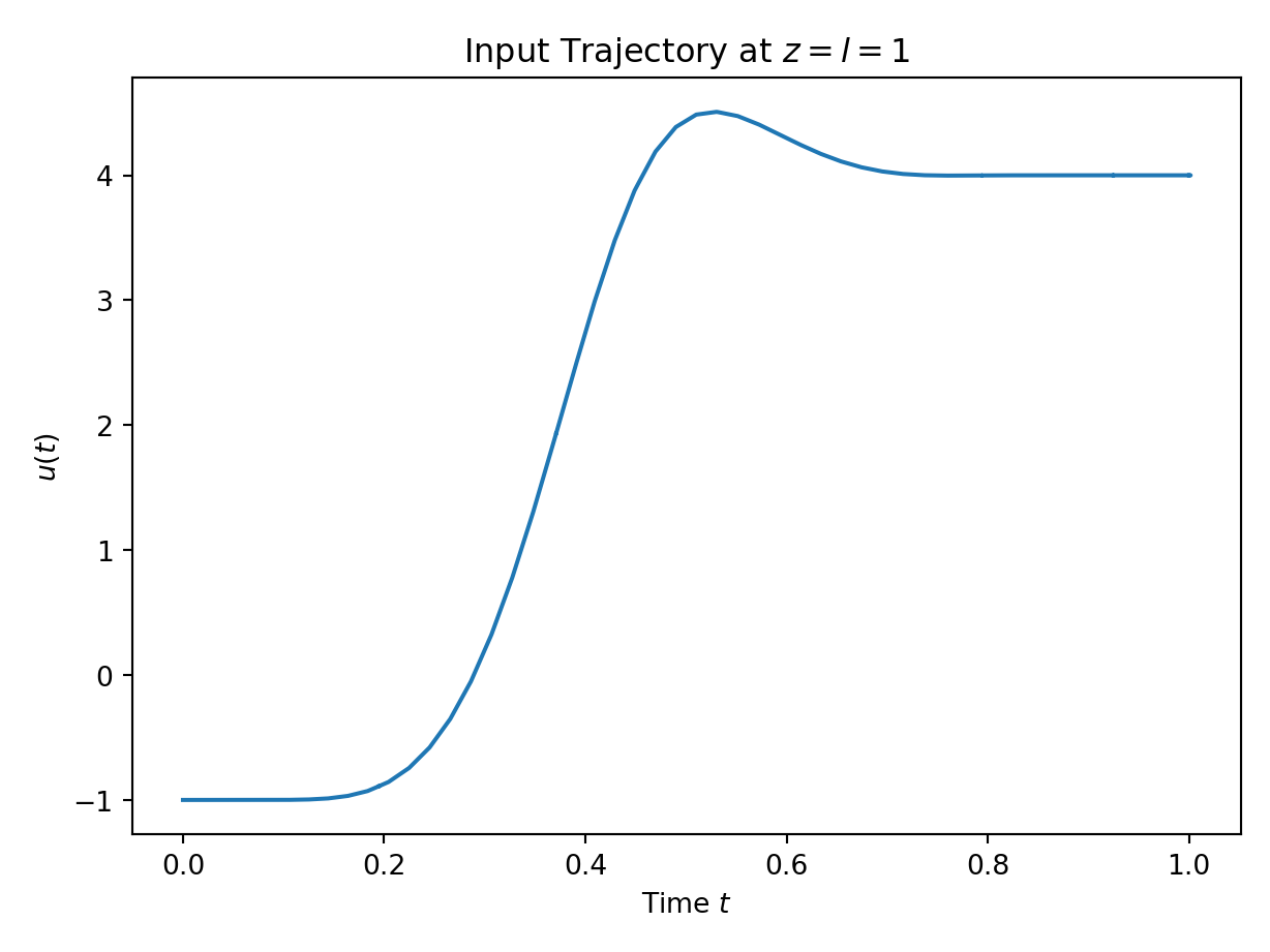
    plt.plot(simulation_data.u._time_storage, simulation_data.u.get_results(simulation_data.u._time_storage))
    plt.xlabel("Time $t$")
    plt.ylabel("$u(t)$")
    plt.title("Input Trajectory at $z=l=1$")
    plt.grid()
    plt.tight_layout()
    save_plot_in_dir("plot_1.png")

    win0 = pi.surface_plot(simulation_data.eval_d, zlabel="x(z,t)")
    plt.title("Temperature Development in Time and Space")
    plt.ylabel("Time $t$")
    plt.xlabel("Space $z$")
    plt.tight_layout()
    save_plot_in_dir("plot_2.png")

    # win2 = pi.PgAnimatedPlot(simulation_data.eval_d,
    #                          labels=dict(left='x(z,t)', bottom='z'))

    # win3 = pi.PgAnimatedPlot(simulation_data.der_eval_d,
    #                          labels=dict(left='x\'(z,t)', bottom='z'))

    # pi.show()


def evaluate_simulation(simulation_data):
    """
    assert that the simulation results are as expected

    :param simulation_data: simulation_data of system_model
    :return:
    """
    expected_final_state = np.array(
        [
            0.0,
            0.02150636,
            0.04301272,
            0.06451907,
            0.08602543,
            0.10753179,
            0.12903815,
            0.1505445,
            0.17205086,
            0.19355722,
            0.21506358,
            0.23656994,
            0.25807628,
            0.27958259,
            0.3010889,
            0.32259522,
            0.34410153,
            0.36560784,
            0.38711415,
            0.40862047,
            0.43012678,
            0.45163309,
            0.47313941,
            0.49464572,
            0.51615199,
            0.53765824,
            0.55916449,
            0.58067075,
            0.602177,
            0.62368325,
            0.64518951,
            0.66669576,
            0.68820201,
            0.70970826,
            0.73121452,
            0.75272075,
            0.77422688,
            0.79573301,
            0.81723913,
            0.83874526,
            0.86025138,
            0.88175751,
            0.90326363,
            0.92476976,
            0.94627588,
            0.96778201,
            0.98928813,
            1.0107942,
            1.03230022,
            1.05380623,
            1.07531225,
            1.09681826,
            1.11832428,
            1.13983029,
            1.16133631,
            1.18284232,
            1.20434834,
            1.22585435,
            1.24736037,
            1.26886621,
            1.29037204,
            1.31187786,
            1.33338368,
            1.35488951,
            1.37639533,
            1.39790116,
            1.41940698,
            1.4409128,
            1.46241863,
            1.48392445,
            1.50543024,
            1.52693592,
            1.5484416,
            1.56994728,
            1.59145296,
            1.61295863,
            1.63446431,
            1.65596999,
            1.67747567,
            1.69898135,
            1.72048703,
            1.74199271,
            1.76349825,
            1.7850037,
            1.80650916,
            1.82801461,
            1.84952007,
            1.87102552,
            1.89253097,
            1.91403643,
            1.93554188,
            1.95704734,
            1.97855279,
            2.00005824,
            2.02156354,
            2.04306884,
            2.06457414,
            2.08607943,
            2.10758473,
            2.12909003,
            2.15059533,
            2.17210063,
            2.19360592,
            2.21511122,
            2.23661652,
            2.25812173,
            2.27962681,
            2.30113188,
            2.32263695,
            2.34414202,
            2.3656471,
            2.38715217,
            2.40865724,
            2.43016232,
            2.45166739,
            2.47317246,
            2.49467753,
            2.5161825,
            2.53768743,
            2.55919236,
            2.58069728,
            2.60220221,
            2.62370714,
            2.64521207,
            2.666717,
            2.68822193,
            2.70972686,
            2.73123178,
            2.75273669,
            2.77424143,
            2.79574616,
            2.8172509,
            2.83875564,
            2.86026038,
            2.88176512,
            2.90326985,
            2.92477459,
            2.94627933,
            2.96778407,
            2.9892888,
            3.01079349,
            3.03229811,
            3.05380274,
            3.07530737,
            3.096812,
            3.11831662,
            3.13982125,
            3.16132588,
            3.18283051,
            3.20433513,
            3.22583976,
            3.24734439,
            3.26884891,
            3.29035341,
            3.31185791,
            3.33336241,
            3.35486691,
            3.37637141,
            3.39787591,
            3.41938041,
            3.44088491,
            3.46238941,
            3.48389391,
            3.50539839,
            3.52690283,
            3.54840727,
            3.56991171,
            3.59141615,
            3.61292059,
            3.63442503,
            3.65592947,
            3.67743391,
            3.69893835,
            3.72044279,
            3.74194724,
            3.76345165,
            3.78495604,
            3.80646044,
            3.82796483,
            3.84946923,
            3.87097363,
            3.89247802,
            3.91398242,
            3.93548681,
            3.95699121,
            3.9784956,
            4.0,
        ]
    )

    rc = ResultContainer(score=1.0)
    simulated_final_state = simulation_data.eval_d.output_data[-1]
    rc.final_state_errors = [
        simulated_final_state[i] - expected_final_state[i] for i in np.arange(0, len(simulated_final_state))
    ]
    rc.success = np.allclose(expected_final_state, simulated_final_state, rtol=0, atol=1e-2)

    return rc

import numpy as np
import pyinduct as pi
import pyinduct.parabolic as parabolic
import matplotlib.pyplot as plt
from ipydex import IPS


def run(show_plots):
    n_fem = 17
    T = 1
    l = 1
    y0 = -1
    y1 = 4

    param = [1, 0, 0, None, None]
    # or try these:
    # param = [1, -0.5, -8, None, None]   #  :)))
    a2, a1, a0, _, _ = param

    temp_domain = pi.Domain(bounds=(0, T), num=100)
    spat_domain = pi.Domain(bounds=(0, l), num=n_fem * 11)

    # initial and test functions
    nodes = pi.Domain(spat_domain.bounds, num=n_fem)
    fem_base = pi.LagrangeFirstOrder.cure_interval(nodes)
    act_fem_base = pi.Base(fem_base[-1])
    not_act_fem_base = pi.Base(fem_base[1:-1])
    vis_fems_base = pi.Base(fem_base)

    pi.register_base("act_base", act_fem_base)
    pi.register_base("sim_base", not_act_fem_base)
    pi.register_base("vis_base", vis_fems_base)

    # trajectory
    u = parabolic.RadFeedForward(
        l, T, param_original=param, bound_cond_type="dirichlet", actuation_type="dirichlet", y_start=y0, y_end=y1
    )

    # weak form
    x = pi.FieldVariable("sim_base")
    x_dt = x.derive(temp_order=1)
    x_dz = x.derive(spat_order=1)
    phi = pi.TestFunction("sim_base")
    phi_dz = phi.derive(1)
    act_phi = pi.ScalarFunction("act_base")
    act_phi_dz = act_phi.derive(1)
    # weak formulation of the PDE equations (see documentation)
    weak_form = pi.WeakFormulation(
        [
            # ... of the homogeneous part of the system
            pi.IntegralTerm(pi.Product(x_dt, phi), limits=spat_domain.bounds),
            pi.IntegralTerm(pi.Product(x_dz, phi_dz), limits=spat_domain.bounds, scale=a2),
            pi.IntegralTerm(pi.Product(x_dz, phi), limits=spat_domain.bounds, scale=-a1),
            pi.IntegralTerm(pi.Product(x, phi), limits=spat_domain.bounds, scale=-a0),
            # ... of the inhomogeneous part of the system
            pi.IntegralTerm(pi.Product(pi.Product(act_phi, phi), pi.Input(u, order=1)), limits=spat_domain.bounds),
            pi.IntegralTerm(
                pi.Product(pi.Product(act_phi_dz, phi_dz), pi.Input(u)), limits=spat_domain.bounds, scale=a2
            ),
            pi.IntegralTerm(pi.Product(pi.Product(act_phi_dz, phi), pi.Input(u)), limits=spat_domain.bounds, scale=-a1),
            pi.IntegralTerm(pi.Product(pi.Product(act_phi, phi), pi.Input(u)), limits=spat_domain.bounds, scale=-a0),
        ],
        name="main_system",
    )

    # system matrices \dot x = A x + b0 u + b1 \dot u
    cf = pi.parse_weak_formulation(weak_form)
    ss = pi.create_state_space(cf)

    a_mat = ss.A[1]
    b0 = ss.B[0][1]
    b1 = ss.B[1][1]

    # transformation into \dot \bar x = \bar A \bar x + \bar b u
    a_tilde = np.diag(np.ones(a_mat.shape[0]), 0)
    a_tilde_inv = np.linalg.inv(a_tilde)

    a_bar = (a_tilde @ a_mat) @ a_tilde_inv
    b_bar = a_tilde @ (a_mat @ b1) + b0

    # simulation
    def x0(z):
        return 0 + y0 * z

    start_func = pi.Function(x0, domain=spat_domain.bounds)
    full_start_state = np.array([pi.project_on_base(start_func, pi.get_base("vis_base"))]).flatten()
    initial_state = full_start_state[1:-1]

    start_state_bar = a_tilde @ initial_state - (b1 * u(time=0)).flatten()
    ss = pi.StateSpace(a_bar, b_bar, base_lbl="sim", input_handle=u)
    sim_temp_domain, sim_weights_bar = pi.simulate_state_space(ss, start_state_bar, temp_domain)

    # back-transformation
    u_vec = np.reshape(u.get_results(sim_temp_domain), (len(temp_domain), 1))
    sim_weights = sim_weights_bar @ a_tilde_inv + u_vec @ b1.T

    # visualisation
    plots = list()
    save_pics = False
    vis_weights = np.hstack((np.zeros_like(u_vec), sim_weights, u_vec))

    eval_d = pi.evaluate_approximation("vis_base", vis_weights, sim_temp_domain, spat_domain, spat_order=0)
    der_eval_d = pi.evaluate_approximation("vis_base", vis_weights, sim_temp_domain, spat_domain, spat_order=1)

    if show_plots:
        plots.append(pi.PgAnimatedPlot(eval_d,
                                 labels=dict(left='x(z,t)', bottom='z'),
                                 save_pics=save_pics))
        # plots.append(pi.PgAnimatedPlot(der_eval_d,
        #                          labels=dict(left='x\'(z,t)', bottom='z'),
        #                          save_pics=save_pics))

        win1 = pi.surface_plot(eval_d, zlabel="x(z,t)")
        # win2 = pi.surface_plot(der_eval_d, title="x'(z,t)")

        
            # win1.gl_widget.grabFrameBuffer().save(path + "rad_dirichlet_3d_x.png")
            # win2.gl_widget.grabFrameBuffer().save(path + 'rad_dirichlet_3d_dx.png')
        # pi.show()
        plt.show()

    pi.tear_down(("act_base", "sim_base", "vis_base"))


if __name__ == "__main__":
    run(True)

import sympy as sp
import symbtools as st
import importlib
import sys, os
import pyinduct as pi
import pyinduct.parabolic as parabolic
import numpy as np
from ipydex import IPS, activate_ips_on_exception

from ackrep_core.system_model_management import GenericModel, import_parameters


class Model:

    # Import parameter_file
    params = import_parameters()
    a2 = [float(i[1]) for i in params.get_default_parameters().items()][0]

    n_fem = 17
    l = 1
    T = 1

    # start and end of input trajectory
    y0 = -1
    y1 = 4

    # coefs of pde
    coefs = [1, 0, 0, None, None]
    # or try these:
    # coefs = [1, -0.5, -8, None, None]
    _, a1, a0, _, _ = coefs

    temp_domain = pi.Domain(bounds=(0, T), num=100)
    spat_domain = pi.Domain(bounds=(0, l), num=n_fem * 11)

    # initial and test functions
    nodes = pi.Domain(spat_domain.bounds, num=n_fem)
    fem_base = pi.LagrangeFirstOrder.cure_interval(nodes)
    act_fem_base = pi.Base(fem_base[-1])
    not_act_fem_base = pi.Base(fem_base[1:-1])
    vis_fems_base = pi.Base(fem_base)

    pi.register_base("act_base", act_fem_base)
    pi.register_base("sim_base", not_act_fem_base)
    pi.register_base("vis_base", vis_fems_base)

    # trajectory
    u = parabolic.RadFeedForward(
        l, T, param_original=coefs, bound_cond_type="dirichlet", actuation_type="dirichlet", y_start=y0, y_end=y1
    )

    # weak form
    x = pi.FieldVariable("sim_base")
    x_dt = x.derive(temp_order=1)
    x_dz = x.derive(spat_order=1)
    phi = pi.TestFunction("sim_base")
    phi_dz = phi.derive(1)
    act_phi = pi.ScalarFunction("act_base")
    act_phi_dz = act_phi.derive(1)
    # weak formulation of the PDE equations (see documentation)
    weak_form = pi.WeakFormulation(
        [
            # ... of the homogeneous part of the system
            pi.IntegralTerm(pi.Product(x_dt, phi), limits=spat_domain.bounds),
            pi.IntegralTerm(pi.Product(x_dz, phi_dz), limits=spat_domain.bounds, scale=a2),
            pi.IntegralTerm(pi.Product(x_dz, phi), limits=spat_domain.bounds, scale=-a1),
            pi.IntegralTerm(pi.Product(x, phi), limits=spat_domain.bounds, scale=-a0),
            # ... of the inhomogeneous part of the system
            pi.IntegralTerm(pi.Product(pi.Product(act_phi, phi), pi.Input(u, order=1)), limits=spat_domain.bounds),
            pi.IntegralTerm(
                pi.Product(pi.Product(act_phi_dz, phi_dz), pi.Input(u)), limits=spat_domain.bounds, scale=a2
            ),
            pi.IntegralTerm(pi.Product(pi.Product(act_phi_dz, phi), pi.Input(u)), limits=spat_domain.bounds, scale=-a1),
            pi.IntegralTerm(pi.Product(pi.Product(act_phi, phi), pi.Input(u)), limits=spat_domain.bounds, scale=-a0),
        ],
        name="main_system",
    )

    # system matrices \dot x = A x + b0 u + b1 \dot u
    cf = pi.parse_weak_formulation(weak_form)
    ss = pi.create_state_space(cf)

    a_mat = ss.A[1]
    b0 = ss.B[0][1]
    b1 = ss.B[1][1]

    # transformation into \dot \bar x = \bar A \bar x + \bar b u
    a_tilde = np.diag(np.ones(a_mat.shape[0]), 0)
    a_tilde_inv = np.linalg.inv(a_tilde)

    a_bar = (a_tilde @ a_mat) @ a_tilde_inv
    b_bar = a_tilde @ (a_mat @ b1) + b0

# -*- coding: utf-8 -*-
"""
Created on Fri Jun 11 13:51:06 2021

@author: Jonathan Rockstroh
"""
import sys
import os
import numpy as np
import sympy as sp

import tabulate as tab


# tailing "_nv" stands for "numerical value"


model_name = "Heat_Equation"

# CREATE SYMBOLIC PARAMETERS
pp_symb = [alpha] = [sp.symbols("alpha", real=True)]


# SYMBOLIC PARAMETER FUNCTIONS
alpha_sf = 1


# List of symbolic parameter functions
pp_sf = [alpha_sf]


# List for Substitution
pp_subs_list = []

# OPTONAL: Dictionary which defines how certain variables shall be written
# in the tabular - key: Symbolic Variable, Value: LaTeX Representation/Code
# useful for example for complex variables: {Z: r"\underline{Z}"}
latex_names = {alpha: r"\alpha"}


# ---------- CREATE BEGIN OF LATEX TABULAR
# Define tabular Header

# DON'T CHANGE FOLLOWING ENTRIES: "Symbol", "Value"
tabular_header = ["Parameter Name", "Symbol", "Value"]

# Define column text alignments
col_alignment = ["left", "center", "center"]

# Define Entries of all columns before the Symbol-Column
# --- Entries need to be latex code
col_1 = ["thermal diffusivity"]

# contains all lists of the columns before the "Symbol" Column
# --- Empty list, if there are no columns before the "Symbol" Column
start_columns_list = [col_1]


# contains all lists of columns after the FIX ENTRIES
# --- Empty list, if there are no columns after the "Value" column
end_columns_list = []