Automatic Control Knowledge Repository
You currently have javascript disabled. Some features will be unavailable. Please consider enabling javascript.Details for: "wave equation 1D"
Name: wave equation 1D
(Key: IKNYP)
Path: ackrep_data/system_models/wave_equation View on GitHub
Type: system_model
Short Description: PDE describing the one-dimensional propagation of a wave
Created: 04.08.2022
Compatible Environment: default_conda_environment (Key: CDAMA)
Source Code [ / ] simulation.py
Related Problems:
Extensive Material:
Download pdf
Result: Script Error.
Last Build: Checkout CI Build
Runtime: 2.3 (estimated: 20s)
The image of the latest CI job is not available. This is a fallback image.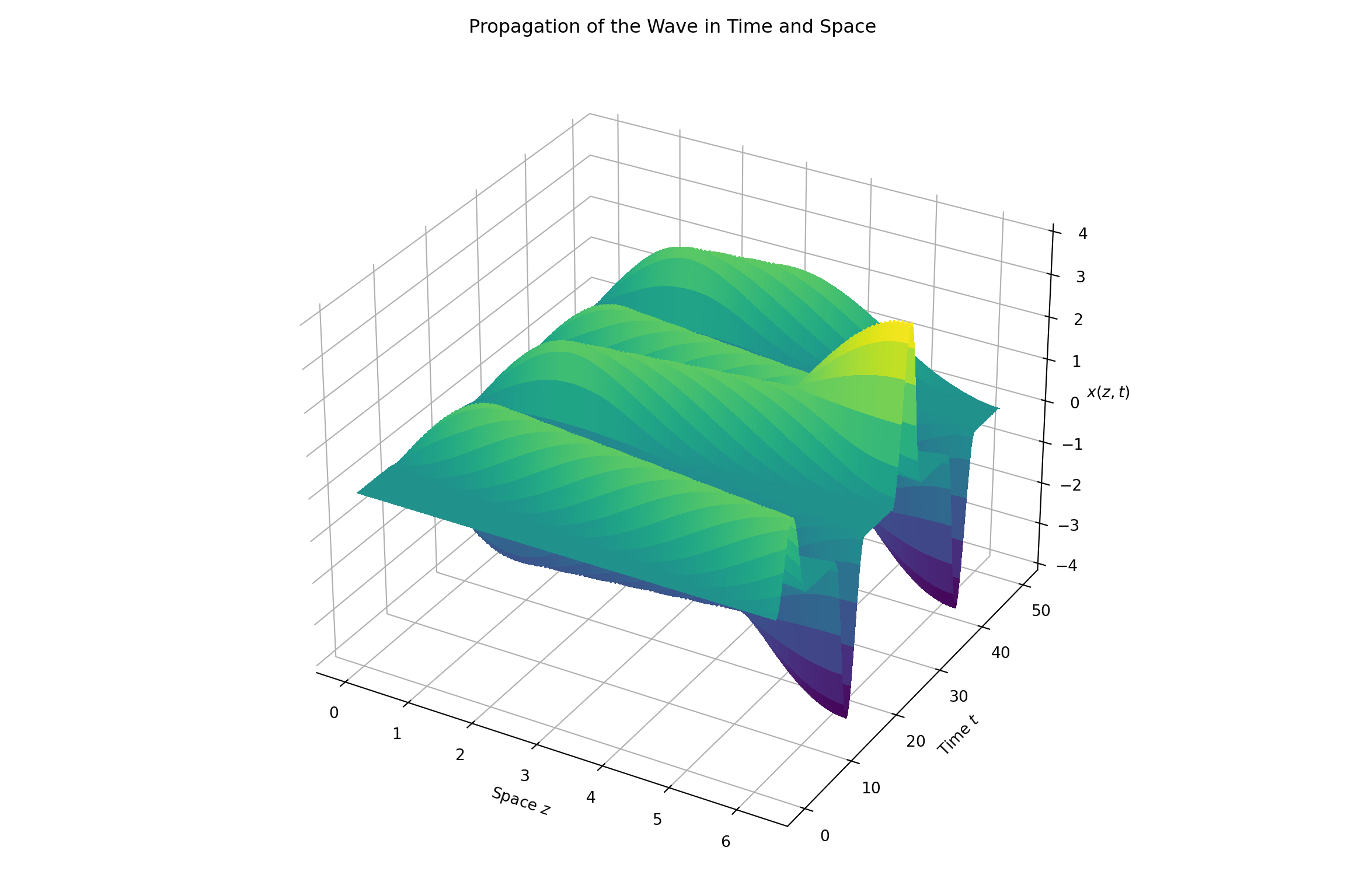
The image of the latest CI job is not available. This is a fallback image. Debug:
Path: ackrep_data/system_models/wave_equation View on GitHub
Type: system_model
Short Description: PDE describing the one-dimensional propagation of a wave
Created: 04.08.2022
Compatible Environment: default_conda_environment (Key: CDAMA)
Source Code [ / ] simulation.py
import numpy as np
import pyinduct as pi
import pyqtgraph as pg
import system_model
from scipy.integrate import solve_ivp
from ackrep_core import ResultContainer
from ackrep_core.system_model_management import save_plot_in_dir
import matplotlib.pyplot as plt
import matplotlib
import os
from ipydex import IPS
# link to documentation with examples: https://ackrep-doc.readthedocs.io/en/latest/devdoc/contributing_data.html
def simulate():
"""
simulate the system model with scipy.integrate.solve_ivp
:return: result of solve_ivp, might contains input function
"""
model = system_model.Model()
print(">>> derive initial conditions")
q0 = pi.core.project_on_bases(model.initial_states, model.canonical_equations)
print(">>> perform time step integration")
sim_domain, q = pi.simulate_state_space(model.state_space_form, q0, model.temp_domain, settings=None)
print(">>> perform postprocessing")
eval_data = pi.get_sim_results(
sim_domain, model.spatial_domains, q, model.state_space_form, derivative_orders=model.derivative_orders
)
evald_x = pi.evaluate_approximation(model.func_label, q[:, : model.n], sim_domain, model.spat_domain, name="x(z,t)")
pi.tear_down(labels=(model.func_label,))
sim = ResultContainer()
sim.u = model.u.get_results(eval_data[0].input_data[0]).flatten()
sim.eval_data = eval_data
sim.evald_x = evald_x
save_plot(sim)
return sim
def save_plot(simulation_data):
"""
plot your data and save the plot
access to data via: simulation_data.t array of time values
simulation_data.y array of data components
simulation_data.uu array of input values
:param simulation_data: simulation_data of system_model
:return: None
"""
# Note: plotting in pyinduct is usually done with pyqtgraph which causes issues during CI.
# This is why the plotting part doesnt look as clean.
# Pyinduct has its own plotting methods, feel free to use them in your own implementation.
matplotlib.use("Agg")
# input visualization
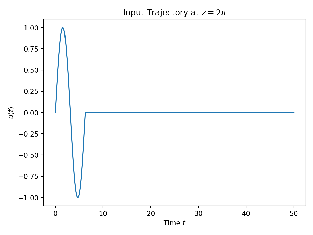
win0 = plt.plot(np.array(simulation_data.eval_data[0].input_data[0]).flatten(), simulation_data.u)
plt.title("Input Trajectory at $z=2\pi$")
plt.xlabel("Time $t$")
plt.ylabel("$u(t)$")
plt.tight_layout()
plt.grid()
save_plot_in_dir("plot_1.png")
win1 = pi.surface_plot(simulation_data.evald_x, zlabel="$x(z,t)$")
plt.title("Propagation of the Wave in Time and Space")
plt.ylabel("Time $t$")
plt.xlabel("Space $z$")
plt.tight_layout()
save_plot_in_dir("plot_2.png")
# vis.save_2d_pg_plot(win0, 'transport_system')
# win1 = pi.PgAnimatedPlot(simulation_data.eval_data,
# title=simulation_data.eval_data[0].name,
# save_pics=False,
# labels=dict(left='x(z,t)', bottom='z'))
# pi.show()
def evaluate_simulation(simulation_data):
"""
assert that the simulation results are as expected
:param simulation_data: simulation_data of system_model
:return:
"""
expected_final_state = np.array(
[
-0.00499123,
0.00998247,
0.02509866,
0.04167615,
0.05997688,
0.08077127,
0.1049973,
0.13320243,
0.16511553,
0.20080206,
0.24051338,
0.28455143,
0.33169568,
0.38166332,
0.4345756,
0.48950293,
0.54560654,
0.60265054,
0.66059809,
0.7191791,
0.77863313,
0.83889479,
0.90044527,
0.96326604,
1.02625365,
1.08924296,
1.15218586,
1.21474135,
1.27650887,
1.33697007,
1.39539469,
1.4512837,
1.50533233,
1.55766056,
1.60842412,
1.65739483,
1.70426427,
1.74852285,
1.78923102,
1.82615575,
1.8593328,
1.88908859,
1.91531896,
1.93833024,
1.95859756,
1.97552569,
1.98838818,
1.99653955,
2.00014191,
1.99954084,
1.99504644,
1.98740683,
1.97630684,
1.96149697,
1.94305579,
1.9208185,
1.89439842,
1.863304,
1.8285013,
1.79124462,
1.7517036,
1.70961109,
1.66492066,
1.61726217,
1.56689181,
1.51390145,
1.45842196,
1.40085832,
1.34170291,
1.28171429,
1.22104533,
1.15970548,
1.0978266,
1.03579091,
0.97373471,
0.91219186,
0.85053241,
0.78807755,
0.72575174,
0.66438022,
0.60454764,
0.54669319,
0.4912745,
0.43833473,
0.38835524,
0.34127898,
0.29700688,
0.25579216,
0.21756052,
0.18142819,
0.14731514,
0.11535209,
0.085886,
0.05901843,
0.03463059,
0.01302813,
-0.00517915,
-0.01954857,
-0.03013463,
-0.03678862,
-0.03905366,
]
)
rc = ResultContainer(score=1.0)
simulated_final_state = simulation_data.eval_data[0].output_data[-1]
rc.final_state_errors = [
simulated_final_state[i] - expected_final_state[i] for i in np.arange(0, len(simulated_final_state))
]
rc.success = np.allclose(expected_final_state, simulated_final_state, rtol=0, atol=1e-2)
return rc
import pyinduct as pi
import numpy as np
import pyqtgraph as pg
from ipydex import IPS

class TestInput(pi.SimulationInput):
    def _calc_output(self, **kwargs):
        t = kwargs["time"]
        if t < 2*np.pi:
            u = np.sin(t)
        else:
            u = 0

        return {"output": u}


sys_name = 'wave equation'
c = 1
l = 2*np.pi
T = 50
n = 101
spat_bounds = (0, l)
spat_domain = pi.Domain(bounds=spat_bounds, num=n)
temp_domain = pi.Domain(bounds=(0, T), num=1000)

# init_x = pi.Function(lambda z: 0, domain=spat_bounds)
def ini(z):
    if z < np.pi:
        u = np.sin(z)
    else:
        u = 0
    return u
init_x_dt = pi.Function(lambda z: 0, domain=spat_bounds)
# init_x_dt = pi.Function(ini, domain=spat_bounds)
init_x = pi.ConstantFunction(0, domain=spat_bounds)


init_funcs = pi.LagrangeFirstOrder.cure_interval(spat_domain)
func_label = 'init_funcs'
pi.register_base(func_label, init_funcs)

u = TestInput("input")
x = pi.FieldVariable(func_label)
phi = pi.TestFunction(func_label)
weak_form = pi.WeakFormulation([
    pi.IntegralTerm(pi.Product(x.derive(temp_order=2), phi), spat_bounds, scale=c**2),
    pi.ScalarTerm(pi.Product(pi.Input(u), phi(l)), scale=-1),
    # pi.ScalarTerm(pi.Product(x.derive(spat_order=1)(l), phi(l)), scale=-1),
    pi.ScalarTerm(pi.Product(x.derive(spat_order=1)(0), phi(0))),
    pi.IntegralTerm(pi.Product(x.derive(spat_order=1), phi.derive(1)), spat_bounds, scale=1),
], name=sys_name)

initial_states = {weak_form.name: [init_x, init_x_dt]}
spatial_domains = {weak_form.name: spat_domain}
derivative_orders = {weak_form.name: (0, 0)}

weak_forms = pi.sanitize_input([weak_form], pi.WeakFormulation)
print("simulate systems: {}".format([f.name for f in weak_forms]))

print(">>> parse weak formulations")
canonical_equations = pi.parse_weak_formulations(weak_forms)

print(">>> create state space system")
state_space_form = pi.create_state_space(canonical_equations)

# --- simulation ---

print(">>> derive initial conditions")
q0 = pi.core.project_on_bases(initial_states, canonical_equations)

print(">>> perform time step integration")
sim_domain, q = pi.simulate_state_space(state_space_form, q0, temp_domain, settings=None)

q[:,0] = q[:,-1] = 0

print(">>> perform postprocessing")
eval_data = pi.get_sim_results(sim_domain, spatial_domains, q, state_space_form, derivative_orders=derivative_orders)

evald_x = pi.evaluate_approximation(func_label, q[:,:n], sim_domain, spat_domain, name="x(z,t)")
evald_dx = pi.evaluate_approximation(func_label, q[:,:n], sim_domain, spat_domain, spat_order=1, name="x'(z,t)")
# IPS()
pi.tear_down(labels=(func_label,))


# pyqtgraph visualization
# vis.save_2d_pg_plot(win0, 'transport_system')
win1 = pi.PgAnimatedPlot(eval_data,
                            title=eval_data[0].name,
                            # save_pics=True,
                            # create_video=True,
                            labels=dict(left='x(z,t)', bottom='z'))

pi.show()

win0 = pg.plot(np.array(eval_data[0].input_data[0]).flatten(),
                u.get_results(eval_data[0].input_data[0]).flatten(),
                labels=dict(left='u(t)', bottom='t'), pen='b')
win0.showGrid(x=False, y=True, alpha=0.5)
win1 = pi.surface_plot(evald_x, zlabel=evald_x.name)
pi.show()
import matplotlib.pyplot as plt
# win1 = pi.surface_plot(evald_dx, zlabel=evald_dx.name)
plt.show()import sympy as sp
import symbtools as st
import importlib
import sys, os
import pyinduct as pi
import numpy as np
from ipydex import IPS, activate_ips_on_exception
from ackrep_core.system_model_management import GenericModel, import_parameters
class TestInput(pi.SimulationInput):
def _calc_output(self, **kwargs):
t = kwargs["time"]
if t < 2 * np.pi:
u = np.sin(t)
else:
u = 0
return {"output": u}
class Model:
# Import parameter_file
params = import_parameters()
c = [float(i[1]) for i in params.get_default_parameters().items()][0]
sys_name = "wave equation"
T = 50
l = 2 * np.pi
n = 101
spat_bounds = (0, l)
spat_domain = pi.Domain(bounds=spat_bounds, num=n)
temp_domain = pi.Domain(bounds=(0, T), num=1000)
init_x = pi.Function(lambda z: 0, domain=spat_bounds)
init_x_dt = pi.ConstantFunction(0, domain=spat_bounds)
init_funcs = pi.LagrangeFirstOrder.cure_interval(spat_domain)
func_label = "init_funcs"
pi.register_base(func_label, init_funcs, overwrite=True)
u = TestInput("input")
x = pi.FieldVariable(func_label)
phi = pi.TestFunction(func_label)
weak_form = pi.WeakFormulation(
[
pi.IntegralTerm(pi.Product(x.derive(temp_order=2), phi), spat_bounds, scale=c**2),
pi.ScalarTerm(pi.Product(pi.Input(u), phi(l)), scale=-1),
pi.ScalarTerm(pi.Product(x.derive(spat_order=1)(0), phi(0))),
pi.IntegralTerm(pi.Product(x.derive(spat_order=1), phi.derive(1)), spat_bounds, scale=1),
],
name=sys_name,
)
initial_states = {weak_form.name: [init_x, init_x_dt]}
spatial_domains = {weak_form.name: spat_domain}
derivative_orders = {weak_form.name: (0, 0)}
weak_forms = pi.sanitize_input([weak_form], pi.WeakFormulation)
print("simulate systems: {}".format([f.name for f in weak_forms]))
print(">>> parse weak formulations")
canonical_equations = pi.parse_weak_formulations(weak_forms)
print(">>> create state space system")
state_space_form = pi.create_state_space(canonical_equations)
# -*- coding: utf-8 -*-
"""
Created on Fri Jun 11 13:51:06 2021

@author: Jonathan Rockstroh
"""
import sys
import os
import numpy as np
import sympy as sp

import tabulate as tab


# tailing "_nv" stands for "numerical value"


model_name = "Wave_Equation"

# CREATE SYMBOLIC PARAMETERS
pp_symb = [c] = [sp.symbols("c", real=True)]


# SYMBOLIC PARAMETER FUNCTIONS
c_sf = 1


# List of symbolic parameter functions
pp_sf = [c_sf]


# List for Substitution
pp_subs_list = []

# OPTONAL: Dictionary which defines how certain variables shall be written
# in the tabular - key: Symbolic Variable, Value: LaTeX Representation/Code
# useful for example for complex variables: {Z: r"\underline{Z}"}
latex_names = {}


# ---------- CREATE BEGIN OF LATEX TABULAR
# Define tabular Header

# DON'T CHANGE FOLLOWING ENTRIES: "Symbol", "Value"
tabular_header = ["Parameter Name", "Symbol", "Value"]

# Define column text alignments
col_alignment = ["left", "center", "center"]

# Define Entries of all columns before the Symbol-Column
# --- Entries need to be latex code
col_1 = ["propagation speed of the wave"]

# contains all lists of the columns before the "Symbol" Column
# --- Empty list, if there are no columns before the "Symbol" Column
start_columns_list = [col_1]


# contains all lists of columns after the FIX ENTRIES
# --- Empty list, if there are no columns after the "Value" column
end_columns_list = []
Related Problems:
Extensive Material:
Download pdf
Result: Script Error.
Last Build: Checkout CI Build
Runtime: 2.3 (estimated: 20s)
Entity passed last: 2023-07-03 13:14:44
with ackrep_data commit: {'author': 'JuliusFiedler', 'branch': 'develop', 'date': '2023-07-03 13:12:35', 'message': 'fix typos and folder names', 'sha': '180d385f485e4aa0d3df6c7a716fa9d1270dc4f3'}
with ackrep_core commit: {'author': 'JuliusFiedler', 'branch': 'develop', 'date': '2023-07-03 09:44:41', 'message': 'black', 'sha': '2bde08d26afc7227546533ecd58f249d24063462'}
in environment: default_conda_environment:0.1.12
Checkout CI Build
Plot:with ackrep_data commit: {'author': 'JuliusFiedler', 'branch': 'develop', 'date': '2023-07-03 13:12:35', 'message': 'fix typos and folder names', 'sha': '180d385f485e4aa0d3df6c7a716fa9d1270dc4f3'}
with ackrep_core commit: {'author': 'JuliusFiedler', 'branch': 'develop', 'date': '2023-07-03 09:44:41', 'message': 'black', 'sha': '2bde08d26afc7227546533ecd58f249d24063462'}
in environment: default_conda_environment:0.1.12
Checkout CI Build
The image of the latest CI job is not available. This is a fallback image.
The image of the latest CI job is not available. This is a fallback image. Debug:
Checking <SystemModel (pk: 151, key: IKNYP)> "(wave equation 1D, 20s)"
13:04:21 - ackrep - INFO -   ... Creating exec-script ...
13:04:21 - ackrep - INFO - execscript-path: /code/ackrep/ackrep_data/execscript.py
13:04:21 - ackrep - INFO -   ... running exec-script /code/ackrep/ackrep_data/execscript.py ...
13:04:22 - ackrep - ERROR -
        The command `python /code/ackrep/ackrep_data/execscript.py` exited with returncode 1.

        stdout:

        stderr: Traceback (most recent call last):
  File "/code/ackrep/ackrep_data/execscript.py", line 35, in <module>
    import system_model
  File "/code/ackrep/ackrep_data/system_models/wave_equation/system_model.py", line 5, in <module>
    import pyinduct as pi
  File "/opt/conda/lib/python3.8/site-packages/pyinduct/__init__.py", line 17, in <module>
    from .eigenfunctions import *
  File "/opt/conda/lib/python3.8/site-packages/pyinduct/eigenfunctions.py", line 24, in <module>
    from .visualization import visualize_roots
  File "/opt/conda/lib/python3.8/site-packages/pyinduct/visualization.py", line 19, in <module>
    import pyqtgraph.opengl as gl
  File "/opt/conda/lib/python3.8/site-packages/pyqtgraph/opengl/__init__.py", line 1, in <module>
    from . import shaders
  File "/opt/conda/lib/python3.8/site-packages/pyqtgraph/opengl/shaders.py", line 1, in <module>
    from OpenGL.GL import *  # noqa
  File "/opt/conda/lib/python3.8/site-packages/OpenGL/GL/__init__.py", line 4, in <module>
    from OpenGL.GL.VERSION.GL_1_1 import *
  File "/opt/conda/lib/python3.8/site-packages/OpenGL/GL/VERSION/GL_1_1.py", line 14, in <module>
    from OpenGL.raw.GL.VERSION.GL_1_1 import *
  File "/opt/conda/lib/python3.8/site-packages/OpenGL/raw/GL/VERSION/GL_1_1.py", line 7, in <module>
    from OpenGL.raw.GL import _errors
  File "/opt/conda/lib/python3.8/site-packages/OpenGL/raw/GL/_errors.py", line 4, in <module>
    _error_checker = _ErrorChecker( _p, _p.GL.glGetError )
AttributeError: 'NoneType' object has no attribute 'glGetError'


Fail.