Automatic Control Knowledge Repository
You currently have javascript disabled. Some features will be unavailable. Please consider enabling javascript.Details for: "PVTOL with 2 forces"
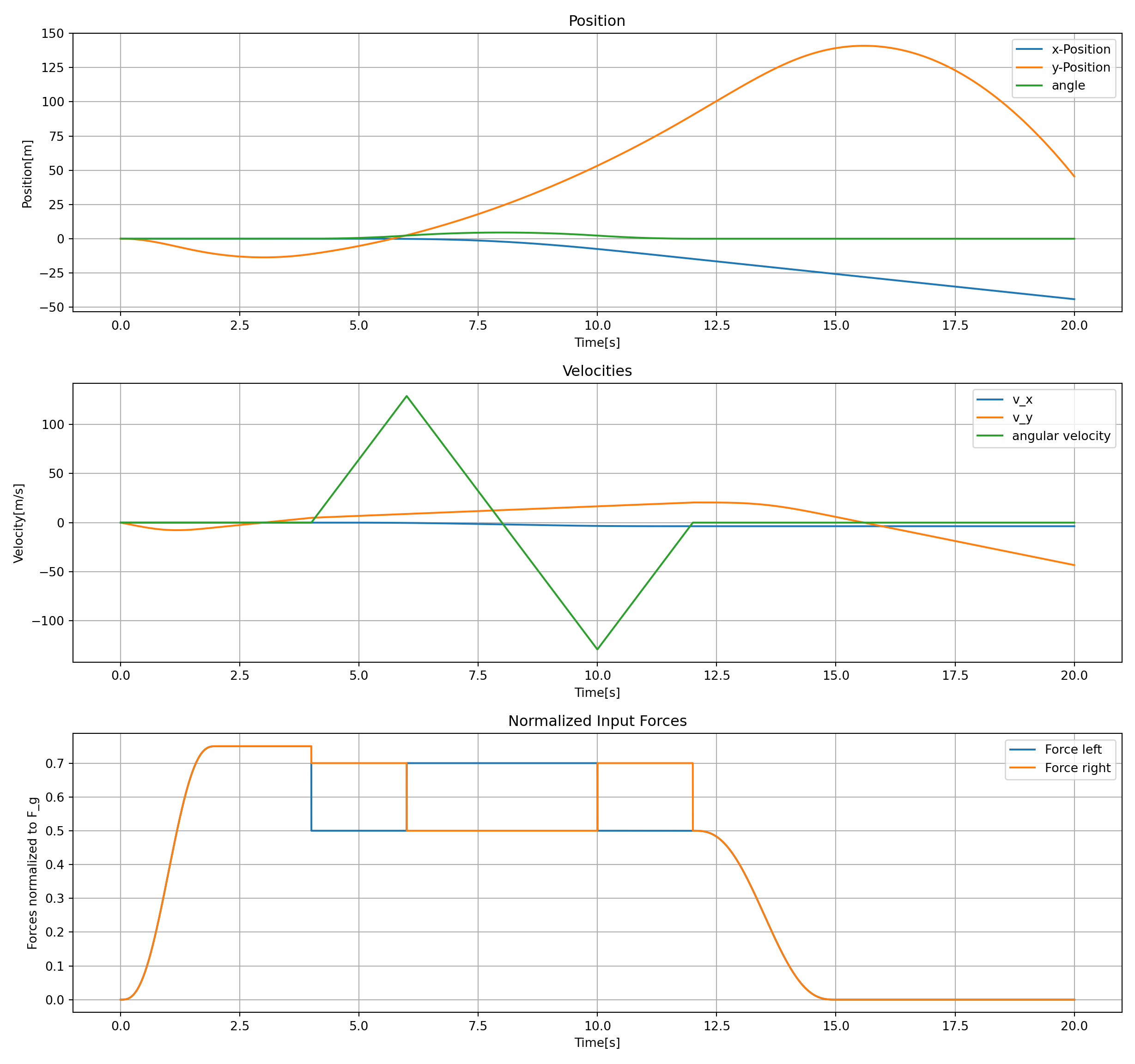
Name: PVTOL with 2 forces
(Key: OHW5Z)
Path: ackrep_data/system_models/pvtol_system View on GitHub
Type: system_model
Short Description: the planar vertical take-off and landing, an underactuated nonlinear unmanned aerial vehicle
Created: 2022-05-09
Compatible Environment: default_conda_environment (Key: CDAMA)
Source Code [ / ] simulation.py
Related Problems:
PVTOL problem
Extensive Material:
Download pdf
Result: Success.
Last Build: Checkout CI Build
Runtime: 7.8 (estimated: 15s)
Plot:
The image of the latest CI job is not available. This is a fallback image.
Path: ackrep_data/system_models/pvtol_system View on GitHub
Type: system_model
Short Description: the planar vertical take-off and landing, an underactuated nonlinear unmanned aerial vehicle
Created: 2022-05-09
Compatible Environment: default_conda_environment (Key: CDAMA)
Source Code [ / ] simulation.py
import numpy as np
import system_model
from scipy.integrate import solve_ivp

from ackrep_core import ResultContainer
from ackrep_core.system_model_management import save_plot_in_dir
import matplotlib.pyplot as plt
import os


def simulate():
    model = system_model.Model()

    rhs_xx_pp_symb = model.get_rhs_symbolic()
    print("Computational Equations:\n")
    for i, eq in enumerate(rhs_xx_pp_symb):
        print(f"dot_x{i+1} =", eq)

    rhs = model.get_rhs_func()

    # Initial State values
    xx0 = np.zeros(6)

    t_end = 20
    tt = np.linspace(0, t_end, 10000)
    sim = solve_ivp(rhs, (0, t_end), xx0, t_eval=tt, max_step=0.01)

    # if inputfunction exists:
    uu = model.uu_func(sim.t, sim.y)
    g = model.get_parameter_value("g")
    m = model.get_parameter_value("m")
    uu = np.array(uu) / (g * m)
    sim.uu = uu

    # --------------------------------------------------------------------

    save_plot(sim)

    return sim


def save_plot(simulation_data):

    # create figure + 2x2 axes array
    fig1, axs = plt.subplots(nrows=3, ncols=1, figsize=(12.8, 12))

    # print in axes top left
    axs[0].plot(simulation_data.t, np.real(simulation_data.y[0]), label="x-Position")
    axs[0].plot(simulation_data.t, np.real(simulation_data.y[2]), label="y-Position")
    axs[0].plot(simulation_data.t, np.real(simulation_data.y[4] * 180 / np.pi), label="angle")
    axs[0].set_title("Position")
    axs[0].set_ylabel("Position [m]")  # y-label Nr 1
    axs[0].set_xlabel("Time [s]")
    axs[0].grid()
    axs[0].legend()

    axs[1].plot(simulation_data.t, simulation_data.y[1], label="$v_x$")
    axs[1].plot(simulation_data.t, simulation_data.y[3], label="$v_y$")
    axs[1].plot(simulation_data.t, simulation_data.y[5] * 180 / np.pi, label="angular velocity")
    axs[1].set_title("Velocities")
    axs[1].set_ylabel("Velocity [m/s]")
    axs[1].set_xlabel("Time [s]")
    axs[1].grid()
    axs[1].legend()

    # print in axes bottom left
    axs[2].plot(simulation_data.t, simulation_data.uu[0], label="Force left")
    axs[2].plot(simulation_data.t, simulation_data.uu[1], label="Force right")
    axs[2].set_title("Normalized Input Forces")
    axs[2].set_ylabel("Forces normalized to $F_g$")  # y-label Nr 1
    axs[2].set_xlabel("Time [s]")
    axs[2].grid()
    axs[2].legend()

    # adjust subplot positioning and show the figure
    fig1.subplots_adjust(hspace=0.5)
    # fig1.show()

    # --------------------------------------------------------------------

    plt.tight_layout()

    save_plot_in_dir()


def evaluate_simulation(simulation_data):
    """

    :param simulation_data: simulation_data of system_model
    :return:
    """
    # fill in the final states y[i][-1] to check your model
    expected_final_state = [
        -44.216119976296774,
        -3.680370979746213,
        45.469521639337344,
        -43.275661598545256,
        -0.00037156407418776797,
        -0.00033632680535548506,
    ]

    # --------------------------------------------------------------------

    rc = ResultContainer(score=1.0)
    simulated_final_state = simulation_data.y[:, -1]
    rc.final_state_errors = [
        simulated_final_state[i] - expected_final_state[i] for i in np.arange(0, len(simulated_final_state))
    ]
    rc.success = np.allclose(expected_final_state, simulated_final_state, rtol=0, atol=1e-2)

    return rc
import sympy as sp
import symbtools as st
import importlib
import sys, os
from ipydex import IPS, activate_ips_on_exception  # for debugging only

from ackrep_core.system_model_management import GenericModel, import_parameters

# Import parameter_file
params = import_parameters()


class Model(GenericModel):
    def initialize(self):
        """
        this function is called by the constructor of GenericModel

        :return: None
        """

        # Define number of inputs -- MODEL DEPENDENT
        self.u_dim = 2

        # Set "sys_dim" to constant value, if system dimension is constant
        # else set "sys_dim" to x_dim -- MODEL DEPENDENT
        self.sys_dim = 6

        # check existance of params file
        self.has_params = True
        self.params = params

    # ----------- SET DEFAULT INPUT FUNCTION ---------- #
    # --------------- Only for non-autonomous Systems
    # --------------- MODEL DEPENDENT

    def uu_default_func(self):
        """
        :param t:(scalar or vector) Time
        :param xx_nv: (vector or array of vectors) state vector with numerical values at time t
        :return:(function with 2 args - t, xx_nv) default input function
        """
        m = self.get_parameter_value("m")
        T_raise = 2
        T_left = T_raise + 2 + 2
        T_right = T_left + 4
        T_straight = T_right + 2
        T_land = T_straight + 3
        force = 0.75 * 9.81 * m
        force_lr = 0.7 * 9.81 * m
        g_nv = 0.5 * self.get_parameter_value("g") * m
        # create symbolic polnomial functions for raise and land
        poly1 = st.condition_poly(self.t_symb, (0, 0, 0, 0), (T_raise, force, 0, 0))

        poly_land = st.condition_poly(self.t_symb, (T_straight, g_nv, 0, 0), (T_land, 0, 0, 0))

        # create symbolic piecewise defined symbolic transition functions
        transition_u1 = st.piece_wise(
            (0, self.t_symb < 0),
            (poly1, self.t_symb < T_raise),
            (force, self.t_symb < T_raise + 2),
            (g_nv, self.t_symb < T_left),
            (force_lr, self.t_symb < T_right),
            (g_nv, self.t_symb < T_straight),
            (poly_land, self.t_symb < T_land),
            (0, True),
        )

        transition_u2 = st.piece_wise(
            (0, self.t_symb < 0),
            (poly1, self.t_symb < T_raise),
            (force, self.t_symb < T_raise + 2),
            (force_lr, self.t_symb < T_left),
            (g_nv, self.t_symb < T_right),
            (force_lr, self.t_symb < T_straight),
            (poly_land, self.t_symb < T_land),
            (0, True),
        )

        # transform symbolic to numeric function
        transition_u1_func = st.expr_to_func(self.t_symb, transition_u1)
        transition_u2_func = st.expr_to_func(self.t_symb, transition_u2)

        def uu_rhs(t, xx_nv):

            u1 = transition_u1_func(t)
            u2 = transition_u2_func(t)

            return [u1, u2]

        return uu_rhs

    # ----------- SYMBOLIC RHS FUNCTION ---------- #
    # --------------- MODEL DEPENDENT

    def get_rhs_symbolic(self):
        """
        :return:(matrix) symbolic rhs-functions
        """
        if self.dxx_dt_symb is not None:
            return self.dxx_dt_symb

        x1, x2, x3, x4, x5, x6 = self.xx_symb
        g, l, m, J = self.pp_symb

        # input
        u1, u2 = self.uu_symb

        # create symbolic rhs functions
        dx1_dt = x2
        dx2_dt = -sp.sin(x5) / m * (u1 + u2)
        dx3_dt = x4
        dx4_dt = sp.cos(x5) / m * (u1 + u2) - g
        dx5_dt = x6 * 2 * sp.pi / 360
        dx6_dt = l / J * (u2 - u1) * 2 * sp.pi / 360

        # put rhs functions into a vector
        self.dxx_dt_symb = sp.Matrix([dx1_dt, dx2_dt, dx3_dt, dx4_dt, dx5_dt, dx6_dt])

        return self.dxx_dt_symb
import sys
import os
import numpy as np
import sympy as sp

import tabulate as tab


# tailing "_nv" stands for "numerical value"

# SET MODEL NAME
model_name = "PVTOL with 2 forces"


# CREATE SYMBOLIC PARAMETERS
pp_symb = [g, l, m, J] = sp.symbols("g, l, m, J", real=True)


# SYMBOLIC PARAMETER FUNCTIONS
# parameter values can be constant/fixed values OR set in relation to other parameters (for example: a = 2*b)
g_sf = 9.81
l_sf = 0.1
m_sf = 0.25
J_sf = 0.00076

# List of symbolic parameter functions
pp_sf = [g_sf, l_sf, m_sf, J_sf]

pp_subs_list = []


# OPTONAL: Dictionary which defines how certain variables shall be written
# in the tabular - key: Symbolic Variable, Value: LaTeX Representation/Code
# useful for example for complex variables: {Z: r"\underline{Z}"}
latex_names = {}


# ---------- CREATE BEGIN OF LATEX TABULAR

# Define tabular Header
# DON'T CHANGE FOLLOWING ENTRIES: "Symbol", "Value"
tabular_header = ["Parametername", "Symbol", "Value", "Unit"]

# Define column text alignments
col_alignment = ["left", "center", "left", "center"]


# Define Entries of all columns before the Symbol-Column
# --- Entries need to be latex code
col_1 = ["acceleration due to gravity", "distance of forces to mass center", "mass", "moment of inertia"]

# contains all lists of the columns before the "Symbol" Column
# --- Empty list, if there are no columns before the "Symbol" Column
start_columns_list = [col_1]


# Define Entries of the columns after the Value-Column
# --- Entries need to be latex code
col_4 = [r"$\frac{\mathrm{m}}{\mathrm{s}^2}$", "m", "kg", r"$\mathrm{kg} \cdot \mathrm{m}^2$"]

# contains all lists of columns after the FIX ENTRIES
# --- Empty list, if there are no columns after the "Value" column
end_columns_list = [col_4]
Related Problems:
PVTOL problem
Extensive Material:
Download pdf
Result: Success.
Last Build: Checkout CI Build
Runtime: 7.8 (estimated: 15s)
Plot:
The image of the latest CI job is not available. This is a fallback image.