Automatic Control Knowledge Repository

#!/usr/bin/env python3
# -*- coding: utf-8 -*-
"""
LQR controller design consists of 4 steps:
1. linearize the non-linear system around the equilibrium point.
2. specify weigh matrices
3. calculate state feedback
4. check whether the system have the desired behavior
"""
try:
    import method_LQR as mlqr  # noqa
    import method_system_property as msp  # noqa
except ImportError:
    from method_packages.method_LQR import method_LQR as mlqr
    from method_packages.method_system_property import method_system_property as msp

import matplotlib.pyplot as plt
import symbtools as st
from scipy.integrate import odeint
import sympy as sp
import os
from ackrep_core.system_model_management import save_plot_in_dir

from ipydex import IPS


class SolutionData:
    pass


def rhs_for_simulation(f, g, xx, controller_func):
    """
    # calculate right hand side equation for simulation of the nonlinear system
    :param f: vector field
    :param g: input matrix
    :param xx: states of the system
    :param controller_func: input equation (trajectory)
    :return: rhs: equation that is solved
    """

    # call the class 'SimulationModel' to build the
    # 'right hand side'equation for ode
    sim_mod = st.SimulationModel(f, g, xx)
    rhs_eq = sim_mod.create_simfunction(controller_function=controller_func)

    return rhs_eq


def solve(problem_spec, kwargs=None):
    """the design of a linear full observer is based on a linear system.
    therefore the non-linear system should first be linearized at the beginning
    :param problem_spec: ProblemSpecification object
    :return: solution_data: states and output values of the stabilized system
    """
    sys_f_body = msp.System_Property()  # instance of the class System_Property
    sys_f_body.sys_state = problem_spec.xx  # state of the system
    sys_f_body.tau = problem_spec.u  # inputs of the system

    # original nonlinear system functions
    sys_f_body.n_state_func = problem_spec.rhs()

    # original output functions
    sys_f_body.n_out_func = problem_spec.output_func()
    sys_f_body.eqlbr = problem_spec.eqrt  # equilibrium point

    # linearize nonlinear system around the chosen equilibrium point
    sys_f_body.sys_linerazition(parameter_values=None)
    tuple_system = (sys_f_body.aa, sys_f_body.bb, sys_f_body.cc, sys_f_body.dd)  # system tuple

    # calculate controller function
    LQR_res = mlqr.lqr_method(
        tuple_system, problem_spec.q, problem_spec.r, problem_spec.xx, problem_spec.eqrt, problem_spec.yr, debug=False
    )
    # simulation original nonlinear system with controller
    f = sys_f_body.n_state_func.subs(st.zip0(sys_f_body.tau))  # x_dot = f(x) + g(x) * u
    g = sys_f_body.n_state_func.jacobian(sys_f_body.tau)

    rhs = rhs_for_simulation(f, g, problem_spec.xx, LQR_res.input_func)
    res = odeint(rhs, problem_spec.xx0, problem_spec.tt)

    output_function = sp.lambdify(problem_spec.xx, sys_f_body.n_out_func, modules="numpy")
    yy = output_function(*res.T)

    solution_data = SolutionData()
    solution_data.res = res  # states of system
    solution_data.pre_filter = LQR_res.pre_filter  # pre-filter
    solution_data.state_feedback = LQR_res.state_feedback  # controller gain
    solution_data.poles = LQR_res.poles_lqr
    solution_data.yy = yy[0][0]

    save_plot(problem_spec, solution_data)

    return solution_data


def save_plot(problem_spec, solution_data):
    titles = ["x1", "x2", "x1_dot", "x2_dot"]
    # simulation for LQR
    plt.figure(1)
    for i in range(4):
        plt.subplot(2, 2, i + 1)
        plt.plot(problem_spec.tt, solution_data.res[:, i], color="k", linewidth=1)
        plt.grid(1)
        plt.title(titles[i])
        plt.xlabel("time t/s")
        if i == 0:
            plt.ylabel("position [m]")
        elif i == 1:
            plt.ylabel("angular position [rad]")
        elif i == 2:
            plt.ylabel("velocity [m/s]")
        else:
            plt.ylabel("angular velocity [rad/s]")
    plt.tight_layout()
    save_plot_in_dir("plot1.png")

    plt.figure(2)
    plt.plot(problem_spec.tt, solution_data.yy)
    plt.grid(1)
    plt.xlabel("time [s]")
    plt.ylabel("position [m]")
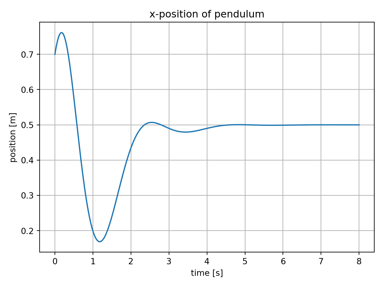
    plt.title("x-position of pendulum")
    plt.tight_layout()

    # save image
    save_plot_in_dir("plot2.png")