Automatic Control Knowledge Repository
You currently have javascript disabled. Some features will be unavailable. Please consider enabling javascript.Details for: "Motion planning for closed kinematic chains using a quasistatic approach"
Name: Motion planning for closed kinematic chains using a quasistatic approach
(Key: Z7HZY)
Path: ackrep_data/problem_solutions/closed_kinematic_chains_quasistatic View on GitHub
Type: problem_solution
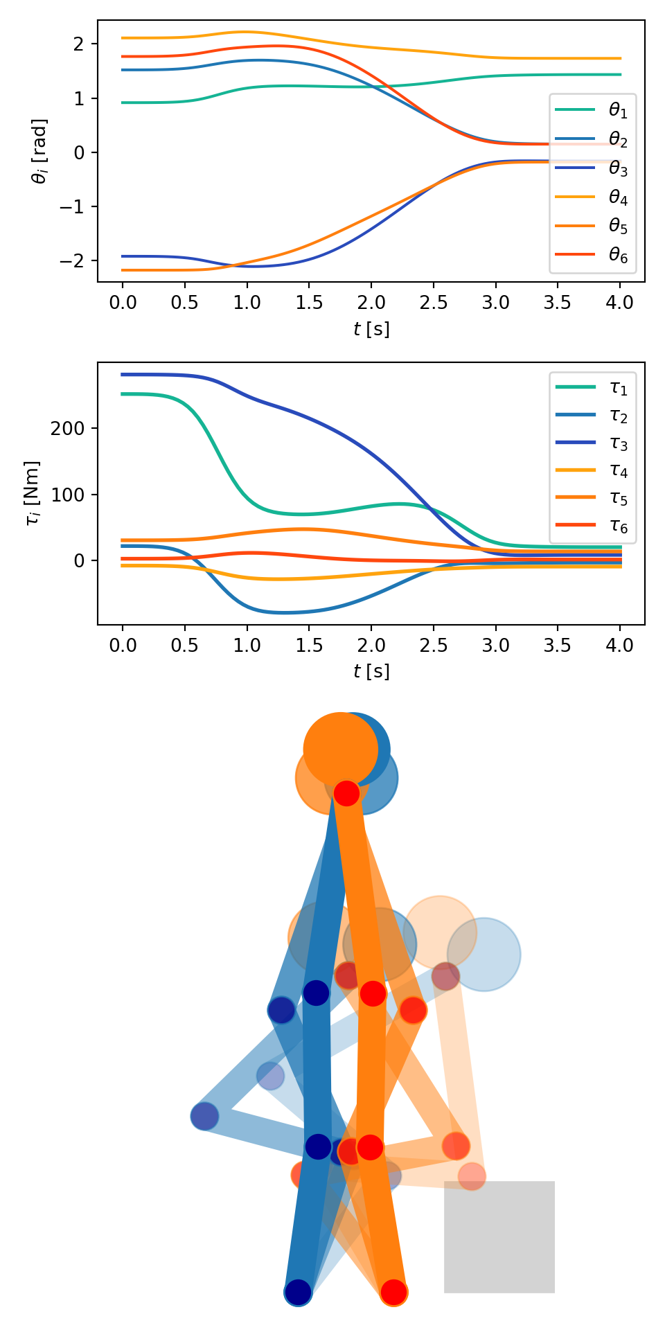
Short Description: Demonstrate motion planning for mechanical closed kinematic chains. The example used is an assisted standing up motion found in geriatric care. Created during supervision of student thesis.
Created:
Compatible Environment: default_conda_environment (Key: CDAMA)
Source Code [ / ] solution.py
Solved Problems: Motion planning for closed kinematic chains |
Used Methods:
Result: Success.
Last Build: Checkout CI Build
Runtime: 13.1 (estimated: 30s)
Plot:
The image of the latest CI job is not available. This is a fallback image.
Path: ackrep_data/problem_solutions/closed_kinematic_chains_quasistatic View on GitHub
Type: problem_solution
Short Description: Demonstrate motion planning for mechanical closed kinematic chains. The example used is an assisted standing up motion found in geriatric care. Created during supervision of student thesis.
Created:
Compatible Environment: default_conda_environment (Key: CDAMA)
Source Code [ / ] solution.py
import numpy as npy
from matplotlib import pyplot as plt, cycler
from matplotlib.gridspec import GridSpec

import symbtools as st
import symbtools.visualisation as vt
import sympy as sp
from symbtools.modeltools import Rz
import symbtools.modeltools as mt
import pickle
import os
import sys
import casadi as cs
import ipydex
from scipy.interpolate import splrep, splev, interp1d

from casadi import SX, inf
import symbtools.mpctools as mpc

from ackrep_core.system_model_management import save_plot_in_dir


class SolutionData:
    pass


def solve(problem_spec):
    # problem_spec is dummy
    t = sp.Symbol("t")  # time variable
    np = 2
    nq = 2
    ns = 2
    n = np + nq + ns

    p1, p2 = pp = st.symb_vector("p1:{0}".format(np + 1))
    q1, q2 = qq = st.symb_vector("q1:{0}".format(nq + 1))
    s1, s2 = ss = st.symb_vector("s1:{0}".format(ns + 1))

    ttheta = st.row_stack(qq[0], pp[0], ss[0], qq[1], pp[1], ss[1])
    qdot1, pdot1, sdot1, qdot2, pdot2, sdot2 = tthetad = st.time_deriv(ttheta, ttheta)
    tthetadd = st.time_deriv(ttheta, ttheta, order=2)

    ttheta_all = st.concat_rows(ttheta, tthetad, tthetadd)

    (
        c1,
        c2,
        c3,
        c4,
        c5,
        c6,
        m1,
        m2,
        m3,
        m4,
        m5,
        m6,
        J1,
        J2,
        J3,
        J4,
        J5,
        J6,
        l1,
        l2,
        l3,
        l4,
        l5,
        l6,
        d,
        g,
    ) = params = sp.symbols(
        "c1, c2, c3, c4, c5, c6, m1, m2, m3, m4, m5, m6, J1, J2, J3, J4, J5, J6, l1, l2, l3, l4, l5, l6, d, g"
    )

    tau1, tau2, tau3, tau4, tau5, tau6 = ttau = st.symb_vector("tau1, tau2, tau3, tau4, tau5, tau6 ")

    # unit vectors

    ex = sp.Matrix([1, 0])
    ey = sp.Matrix([0, 1])

    # coordinates of centers of mass and joints
    # left
    G0 = 0 * ex  ##:

    C1 = G0 + Rz(q1) * ex * c1  ##:

    G1 = G0 + Rz(q1) * ex * l1  ##:

    C2 = G1 + Rz(q1 + p1) * ex * c2  ##:

    G2 = G1 + Rz(q1 + p1) * ex * l2  ##:

    C3 = G2 + Rz(q1 + p1 + s1) * ex * c3  ##:

    G3 = G2 + Rz(q1 + p1 + s1) * ex * l3  ##:

    # right
    G6 = d * ex  ##:

    C6 = G6 + Rz(q2) * ex * c6  ##:

    G5 = G6 + Rz(q2) * ex * l6  ##:

    C5 = G5 + Rz(q2 + p2) * ex * c5  ##:

    G4 = G5 + Rz(q2 + p2) * ex * l5  ##:

    C4 = G4 + Rz(q2 + p2 + s2) * ex * c4  ##:

    G3b = G4 + Rz(q2 + p2 + s2) * ex * l4  ##:

    # time derivatives of centers of mass
    Sd1, Sd2, Sd3, Sd4, Sd5, Sd6 = st.col_split(st.time_deriv(st.col_stack(C1, C2, C3, C4, C5, C6), ttheta))

    # Kinetic Energy (note that angles are relative)

    T_rot = (
        (J1 * qdot1**2) / 2
        + (J2 * (qdot1 + pdot1) ** 2) / 2
        + (J3 * (qdot1 + pdot1 + sdot1) ** 2) / 2
        + (J4 * (qdot2 + pdot2 + sdot2) ** 2) / 2
        + (J5 * (qdot2 + pdot2) ** 2) / 2
        + (J6 * qdot2**2) / 2
    )
    T_trans = (
        m1 * Sd1.T * Sd1 + m2 * Sd2.T * Sd2 + m3 * Sd3.T * Sd3 + m4 * Sd4.T * Sd4 + m5 * Sd5.T * Sd5 + m6 * Sd6.T * Sd6
    ) / 2

    T = T_rot + T_trans[0]

    # Potential Energy
    V = m1 * g * C1[1] + m2 * g * C2[1] + m3 * g * C3[1] + m4 * g * C4[1] + m5 * g * C5[1] + m6 * g * C6[1]
    parameter_values = list(
        dict(
            c1=0.4 / 2,
            c2=0.42 / 2,
            c3=0.55 / 2,
            c4=0.55 / 2,
            c5=0.42 / 2,
            c6=0.4 / 2,
            m1=6.0,
            m2=12.0,
            m3=39.6,
            m4=39.6,
            m5=12.0,
            m6=6.0,
            J1=(6 * 0.4**2) / 12,
            J2=(12 * 0.42**2) / 12,
            J3=(39.6 * 0.55**2) / 12,
            J4=(39.6 * 0.55**2) / 12,
            J5=(12 * 0.42**2) / 12,
            J6=(6 * 0.4**2) / 12,
            l1=0.4,
            l2=0.42,
            l3=0.55,
            l4=0.55,
            l5=0.42,
            l6=0.4,
            d=0.26,
            g=9.81,
        ).items()
    )

    external_forces = [tau1, tau2, tau3, tau4, tau5, tau6]

    dir_of_this_file = os.path.dirname(os.path.abspath(sys.modules.get(__name__).__file__))
    fpath = os.path.join(dir_of_this_file, "7L-dae-2020-07-15.pcl")

    if not os.path.isfile(fpath):
        # if model is not present it could be regenerated
        # however this might take long (approx. 20min)
        mod = mt.generate_symbolic_model(T, V, ttheta, external_forces, constraints=[G3 - G3b], simplify=False)
        mod.calc_state_eq(simplify=False)

        mod.f_sympy = mod.f.subs(parameter_values)
        mod.G_sympy = mod.g.subs(parameter_values)
        with open(fpath, "wb") as pfile:
            pickle.dump(mod, pfile)
    else:
        with open(fpath, "rb") as pfile:
            mod = pickle.load(pfile)

    # calculate DAE equations from symbolic model
    dae = mod.calc_dae_eq(parameter_values)

    dae.generate_eqns_funcs()

    torso1_unit = Rz(q1 + p1 + s1) * ex
    torso2_unit = Rz(q2 + p2 + s2) * ex

    neck_length = 0.12
    head_radius = 0.1

    body_width = 15
    neck_width = 15

    H1 = G3 + neck_length * torso1_unit
    H1r = G3 + (neck_length - head_radius) * torso1_unit
    H2 = G3b + neck_length * torso2_unit
    H2r = G3b + (neck_length - head_radius) * torso2_unit

    vis = vt.Visualiser(ttheta, xlim=(-1.5, 1.5), ylim=(-0.2, 2))

    # get default colors and set them explicitly
    # this prevents color changes in onion skin plot
    default_colors = plt.get_cmap("tab10")
    guy1_color = default_colors(0)
    guy1_joint_color = "darkblue"
    guy2_color = default_colors(1)
    guy2_joint_color = "red"
    guy1_head_fc = guy1_color  # facecolor
    guy1_head_ec = guy1_head_fc  # edgecolor
    guy2_head_fc = guy2_color  # facecolor
    guy2_head_ec = guy2_head_fc  # edgecolor

    # guy 1 body
    vis.add_linkage(
        st.col_stack(G0, G1, G2, G3).subs(parameter_values),
        color=guy1_color,
        solid_capstyle="round",
        lw=body_width,
        ms=body_width,
        mfc=guy1_joint_color,
    )
    # guy 1 neck
    # vis.add_linkage(st.col_stack(G3, H1r).subs(parameter_values), color=head_color, solid_capstyle='round', lw=neck_width)
    # guy 1 head
    vis.add_disk(
        st.col_stack(H1, H1r).subs(parameter_values), fc=guy1_head_fc, ec=guy1_head_ec, plot_radius=False, fill=True
    )

    # guy 2 body
    vis.add_linkage(
        st.col_stack(G6, G5, G4, G3b).subs(parameter_values),
        color=guy2_color,
        solid_capstyle="round",
        lw=body_width,
        ms=body_width,
        mfc=guy2_joint_color,
    )
    # guy 2 neck
    # vis.add_linkage(st.col_stack(G3b, H2r).subs(parameter_values), color=head_color, solid_capstyle='round', lw=neck_width)
    # guy 2 head
    vis.add_disk(
        st.col_stack(H2, H2r).subs(parameter_values), fc=guy2_head_fc, ec=guy2_head_ec, plot_radius=False, fill=True
    )

    eq_stat = mod.eqns.subz0(tthetadd).subz0(tthetad).subs(parameter_values)

    # vector for tau and lambda together

    ttau_symbols = sp.Matrix(mod.uu)  ##:T

    mmu = st.row_stack(ttau_symbols, mod.llmd)  ##:T

    # linear system of equations (and convert to function w.r.t. ttheta)

    K0_expr = eq_stat.subz0(mmu)  ##:i
    K1_expr = eq_stat.jacobian(mmu)  ##:i

    K0_func = st.expr_to_func(ttheta, K0_expr)
    K1_func = st.expr_to_func(ttheta, K1_expr, keep_shape=True)

    def get_mu_stat_for_theta(ttheta_arg, rho=10):
        # weighting matrix for mu

        K0 = K0_func(*ttheta_arg)
        K1 = K1_func(*ttheta_arg)

        return solve_qlp(K0, K1, rho)

    def solve_qlp(K0, K1, rho):
        R_mu = npy.diag([1, 1, 1, rho, rho, rho, 0.1, 0.1])
        n1, n2 = K1.shape

        # construct the equation system for least squares with linear constraints
        M1 = npy.column_stack((R_mu, K1.T))
        M2 = npy.column_stack((K1, npy.zeros((n1, n1))))
        M_coeff = npy.row_stack((M1, M2))

        M_rhs = npy.concatenate((npy.zeros(n2), -K0))

        mmu_stat = npy.linalg.solve(M_coeff, M_rhs)[:n2]
        return mmu_stat

    ttheta_start = npy.r_[0.9, 1.5, -1.9, 2.1, -2.175799453493845, 1.7471971159642905]

    mmu_start = get_mu_stat_for_theta(ttheta_start)

    connection_point_func = st.expr_to_func(ttheta, G3.subs(parameter_values))

    cs_ttau = mpc.casidify(mod.uu, mod.uu)[0]
    cs_llmd = mpc.casidify(mod.llmd, mod.llmd)[0]

    controls_sp = mmu
    controls_cs = cs.vertcat(cs_ttau, cs_llmd)
    coords_cs, _ = mpc.casidify(ttheta, ttheta)

    # parameters: 0: value of y_connection, 1: x_connection_last,
    # 2: y_connection_last, 3: delta_r_max, 4: rho (penalty factor for 2nd persons torques),
    # 5:11: ttheta_old[6], 11:17: ttheta:old2
    #
    P = SX.sym("P", 5 + 12)
    rho = P[10]

    # weightning of inputs
    R = mpc.SX_diag_matrix((1, 1, 1, rho, rho, rho, 0.1, 0.1))

    #  Construction of Constraints

    g1 = []  # constraints vector (system dynamics)
    g2 = []  # inequality-constraints

    closed_chain_constraint, _ = mpc.casidify(mod.dae.constraints, ttheta, cs_vars=coords_cs)
    connection_position, _ = mpc.casidify(list(G3.subs(parameter_values)), ttheta, cs_vars=coords_cs)  ##:i
    connection_y_value, _ = mpc.casidify([G3[1].subs(parameter_values)], ttheta, cs_vars=coords_cs)  ##:i

    stationary_eqns, _, _ = mpc.casidify(eq_stat, ttheta, controls_sp, cs_vars=(coords_cs, controls_cs))  ##:i

    g1.extend(mpc.unpack(stationary_eqns))
    g1.extend(mpc.unpack(closed_chain_constraint))

    # force the connecting joint to a given hight (which will be provided later)
    g1.append(connection_y_value - P[0])

    ng1 = len(g1)

    # squared distance from the last reference should be smaller than P[3] (delta_r_max):
    # this will be a restriction between -inf and 0
    r = connection_position - P[1:3]
    g2.append(r.T @ r - P[3])

    # change of angles should be smaller than a given bound (P[5:11] are the old coords)
    coords_old = P[5:11]
    coords_old2 = P[11:17]
    pseudo_vel = (coords_cs - coords_old) / 1
    pseudo_acc = (coords_cs - 2 * coords_old + coords_old2) / 1

    g2.extend(mpc.unpack(pseudo_vel))
    g2.extend(mpc.unpack(pseudo_acc))

    g_all = mpc.seq_to_SX_matrix(g1 + g2)

    ### Construction of objective Function

    obj = controls_cs.T @ R @ controls_cs + 1e5 * pseudo_acc.T @ pseudo_acc + 0.3e6 * pseudo_vel.T @ pseudo_vel

    OPT_variables = cs.vertcat(coords_cs, controls_cs)

    # for debugging
    g_all_cs_func = cs.Function("g_all_cs_func", (OPT_variables, P), (g_all,))

    nlp_prob = dict(f=obj, x=OPT_variables, g=g_all, p=P)

    ipopt_settings = dict(max_iter=5000, print_level=0, acceptable_tol=1e-8, acceptable_obj_change_tol=1e-6)
    opts = dict(print_time=False, ipopt=ipopt_settings)

    xx_guess = npy.r_[ttheta_start, mmu_start]

    # note: g1 contains the equality constraints (system dynamics) (lower bound = upper bound)

    delta_phi = 0.05
    d_delta_phi = 0.02
    eps = 1e-9
    lbg = npy.r_[[-eps] * ng1 + [-inf] + [-delta_phi] * n, [-d_delta_phi] * n]
    ubg = npy.r_[[eps] * ng1 + [0] + [delta_phi] * n, [d_delta_phi] * n]

    # ubx = [inf]*OPT_variables.shape[0]##:

    # lower and upper bounds for decision variables:
    # lbx = [-inf, -inf, -inf, -inf, -inf, -inf, -inf, -inf]*N1 + [tau1_min, tau4_min, -inf, -inf]*N
    # ubx = [inf, inf, inf, inf, inf, inf, inf, inf]*N1 + [tau1_max, tau4_max, inf, inf]*N

    rho = 3
    P_init = npy.r_[
        connection_point_func(*ttheta_start)[1],
        connection_point_func(*ttheta_start),
        0.01,
        rho,
        ttheta_start,
        ttheta_start,
    ]

    args = dict(
        lbx=-inf,
        ubx=inf,
        lbg=lbg,
        ubg=ubg,  # unconstrained optimization
        p=P_init,  # initial and final state
        x0=xx_guess,  # initial guess
    )

    solver = cs.nlpsol("solver", "ipopt", nlp_prob, opts)
    sol = solver(**args)

    global_vars = ipydex.Container(old_sol=xx_guess, old_sol2=xx_guess)

    def get_optimal_equilibrium(y_value, rho=3):

        ttheta_old = global_vars.old_sol[:n]
        ttheta_old2 = global_vars.old_sol2[:n]
        opt_prob_params = npy.r_[y_value, connection_point_func(*ttheta_old), 0.01, rho, ttheta_old, ttheta_old2]

        args.update(dict(p=opt_prob_params, x0=global_vars.old_sol))
        sol = solver(**args)

        stats = solver.stats()
        if not stats["success"]:
            raise ValueError(stats["return_status"])

        XX = sol["x"].full().squeeze()

        # save the last two results
        global_vars.old_sol2 = global_vars.old_sol
        global_vars.old_sol = XX

        return XX

    y_start = connection_point_func(*ttheta_start)[1]
    N = 100

    y_end = 1.36
    y_func = st.expr_to_func(t, st.condition_poly(t, (0, y_start, 0, 0), (1, y_end, 0, 0)))

    def get_qs_trajectory(rho):
        pseudo_time = npy.linspace(0, 1, N)
        yy_connection = y_func(pseudo_time)

        # reset the initial guess
        global_vars.old_sol = xx_guess
        global_vars.old_sol2 = xx_guess
        XX_list = []
        for i, y_value in enumerate(yy_connection):
            # print(i, y_value)
            XX_list.append(get_optimal_equilibrium(y_value, rho=rho))

        XX = npy.array(XX_list)
        return XX

    rho = 30
    XX = get_qs_trajectory(rho=rho)

    def smooth_time_scaling(Tend, N, phase_fraction=0.5):
        """
        :param Tend:
        :param N:
        :param phase_fraction:   fraction of Tend for smooth initial and end phase
        """

        T0 = 0
        T1 = Tend * phase_fraction

        y0 = 0
        y1 = 1

        # for initial phase
        poly1 = st.condition_poly(t, (T0, y0, 0, 0), (T1, y1, 0, 0))

        # for end phase
        poly2 = poly1.subs(t, Tend - t)

        # there should be a phase in the middle with constant slope
        deriv_transition = st.piece_wise(
            (y0, t < T0), (poly1, t < T1), (y1, t < Tend - T1), (poly2, t < Tend), (y0, True)
        )

        scaling = sp.integrate(deriv_transition, (t, T0, Tend))

        time_transition = sp.integrate(deriv_transition * N / scaling, t)

        # deriv_transition_func = st.expr_to_func(t, full_transition)
        time_transition_func = st.expr_to_func(t, time_transition)
        deriv_func = st.expr_to_func(t, deriv_transition * N / scaling)
        deriv_func2 = st.expr_to_func(t, deriv_transition.diff(t) * N / scaling)

        C = ipydex.Container(fetch_locals=True)

        return C

    N = XX.shape[0]
    Tend = 4
    res = smooth_time_scaling(Tend, N)

    def get_derivatives(XX, time_scaling, res=100):
        """
        :param XX:             Nxm array
        :param time_scaling:   container for time scaling
        :param res:            time resolution of the returned arrays
        """

        N = XX.shape[0]
        Tend = time_scaling.Tend
        assert npy.isclose(time_scaling.time_transition_func([0, Tend])[-1], N)

        tt = npy.linspace(time_scaling.T0, time_scaling.Tend, res)
        NN = npy.arange(N)

        # high_resolution version of index arry
        NN2 = npy.linspace(0, N, res, endpoint=False)

        # time-scaled verion of index-array
        NN3 = time_scaling.time_transition_func(tt)
        NN3d = time_scaling.deriv_func(tt)
        NN3dd = time_scaling.deriv_func2(tt)

        XX_num, XXd_num, XXdd_num = [], [], []

        # iterate over every column
        for col in XX.T:
            spl = splrep(NN, col)

            # function value and derivatives
            XX_num.append(splev(NN3, spl))
            XXd_num.append(splev(NN3, spl, der=1))
            XXdd_num.append(splev(NN3, spl, der=2))

        XX_num = npy.array(XX_num).T
        XXd_num = npy.array(XXd_num).T
        XXdd_num = npy.array(XXdd_num).T

        NN3d_bc = npy.broadcast_to(NN3d, XX_num.T.shape).T
        NN3dd_bc = npy.broadcast_to(NN3dd, XX_num.T.shape).T

        XXd_n = XXd_num * NN3d_bc

        # apply chain rule
        XXdd_n = XXdd_num * NN3d_bc**2 + XXd_num * NN3dd_bc

        C = ipydex.Container(fetch_locals=True)
        return C

    C = XX_derivs = get_derivatives(XX[:, :], time_scaling=res)

    expr = mod.eqns.subz0(mod.uu, mod.llmd).subs(parameter_values)
    dynterm_func = st.expr_to_func(ttheta_all, expr)

    def get_torques(dyn_term_func, XX_derivs, static1=False, static2=False):

        ttheta_num_all = npy.c_[XX_derivs.XX_num[:, :n], XX_derivs.XXd_n[:, :n], XX_derivs.XXdd_n[:, :n]]  ##:S

        if static1:
            # set velocities to 0
            ttheta_num_all[:, n : 2 * n] = 0

        if static2:
            # set accelerations to 0
            ttheta_num_all[:, 2 * n :] = 0

        res = dynterm_func(*ttheta_num_all.T)
        return res

    lhs_static = get_torques(dynterm_func, XX_derivs, static1=True, static2=True)  ##:i
    lhs_dynamic = get_torques(dynterm_func, XX_derivs, static2=False)  ##:i

    mmu_stat_list = []
    for L_k_stat, L_k_dyn, ttheta_k in zip(lhs_static, lhs_dynamic, XX_derivs.XX_num[:, :n]):
        K1_k = K1_func(*ttheta_k)
        mmu_stat_k = solve_qlp(L_k_stat, K1_k, rho)
        mmu_stat_list.append(mmu_stat_k)

    mmu_stat_all = npy.array(mmu_stat_list)

    solution_data = SolutionData()
    solution_data.tt = XX_derivs.tt
    solution_data.xx = XX_derivs.XX_num
    solution_data.mmu = mmu_stat_all
    solution_data.vis = vis

    save_plot(problem_spec, solution_data)

    return solution_data


def save_plot(problem_spec, solution_data):
    color_cycle = cycler(color=["#15B494", "#1F77B4", "#294BBB", "#FFA30E", "#ff7f0e", "#FF480E"])

    fig = plt.figure(figsize=(5, 10))

    grid = GridSpec(4, 1)

    plt.subplot(grid[0, 0])
    plt.gca().set_prop_cycle(color_cycle)
    plt.plot(solution_data.tt, solution_data.xx[:, :6], "-")

    plt.xlabel(r"$t$ [s]")
    plt.ylabel(r"$\theta_i$ [rad]")
    plt.legend(
        ["$\\theta_1$", "$\\theta_2$", "$\\theta_3$", "$\\theta_4$", "$\\theta_5$", "$\\theta_6$"], loc="lower right"
    )

    plt.subplot(grid[1, 0])
    plt.gca().set_prop_cycle(color_cycle)
    plt.plot(solution_data.tt, solution_data.mmu[:, :6], "-", lw=2)

    plt.xlabel(r"$t$ [s]")
    plt.ylabel(r"$\tau_i$ [Nm]")
    plt.legend(["$\\tau_1$", "$\\tau_2$", "$\\tau_3$", "$\\tau_4$", "$\\tau_5$", "$\\tau_6$"])

    frames = [0, 25, 60, 99]

    ttheta_onion = solution_data.xx[:, :6]
    ttheta_onion = ttheta_onion[frames, :]

    _, ax = solution_data.vis.create_default_axes(fig=fig, add_subplot_args=grid[2:, 0])
    ax.grid(False)
    ax.set_axis_off()
    ax.set_xlim(-0.3, 0.7)
    ax.set_ylim(-0.05, 1.6)

    # draw chair
    from matplotlib.patches import Rectangle

    chair = Rectangle((0.4, 0), 1, 0.3, color="lightgray")
    ax.add_patch(chair)

    # plot onion skins
    # change_alpha=True tweaks the alpha channel, change_alpha=False tweaks the color lightness
    solution_data.vis.plot_onion_skinned(ttheta_onion, axes=ax, change_alpha=True, max_lightness=0.75)

    plt.tight_layout()

    save_plot_in_dir()
Solved Problems: Motion planning for closed kinematic chains |
Used Methods:
Result: Success.
Last Build: Checkout CI Build
Runtime: 13.1 (estimated: 30s)
Plot:
The image of the latest CI job is not available. This is a fallback image.